Getting Started with TissueMask

Why spatial masks?

In spatial transcriptomics and spatial proteomics experiments, the tissue of interest occupies an irregular region of the slide. Before computing any spatially-resolved quantity — cell-type composition, signalling gradients, diffusion fields — you need a reliable spatial mask: a polygon or multi-polygon that faithfully represents the shape of the tissue.

fit_spatial_mask() takes a set of XY point coordinates (typically cell centroids or single-molecule transcript locations) and fits a mask polygon to them. It returns an sf geometry object compatible with the broader sf/GEOS/GDAL ecosystem.

Installation

# From GitHub (requires pak or remotes)
pak::pkg_install("RaredonLab/TissueMask")

# Optional method dependencies
install.packages(c("concaveman", "MASS", "isoband", "ggplot2", "patchwork"))

Method overview

`method`	Topology	Speed	Key packages
`"raster"` (default)	Holes + islands	Fast	`sf` only
`"kde"`	Holes + islands	Moderate	`MASS`, `isoband`
`"concave"`	No holes	Fast	`concaveman`
`"convex"`	No holes	Instant	`sf` only

library(TissueMask)
library(sf)
library(ggplot2)

set.seed(42)

Shared plotting helper

We use geom_sf() throughout — not geom_polygon(). This is essential: geom_polygon() draws a line between consecutive rings, producing diagonal artefacts across hole interiors. geom_sf() delegates rendering to the sf/GEOS layer, which handles holes correctly.

plot_mask <- function(mask, coords, title = "", subtitle = "",
                      fill = "#4c9be8", border = "#1a5fa8",
                      pt_col = "#c0392b", pt_size = 1.0, pt_alpha = 0.55) {
  mask_sf <- sf::st_sf(geometry = mask)
  ggplot() +
    geom_sf(data = mask_sf, fill = fill, alpha = 0.2,
            color = border, linewidth = 0.55) +
    geom_point(data = coords, aes(x = x, y = y),
               color = pt_col, size = pt_size, alpha = pt_alpha) +
    coord_sf(datum = NA) +
    labs(title = title, subtitle = subtitle, x = "X", y = "Y") +
    theme_minimal(base_size = 10) +
    theme(plot.title    = element_text(face = "bold", size = 10),
          plot.subtitle = element_text(size = 8, color = "grey40"),
          panel.grid    = element_line(color = "grey93"))
}

1. Convex hull

The convex hull is the tightest convex polygon that contains all points. It is instantaneous and requires only sf, but cannot represent non-convex tissue shapes or internal voids.

# Simple circular cloud
coords_circle <- data.frame(x = rnorm(400, 0, 1), y = rnorm(400, 0, 1))

mask_convex <- fit_spatial_mask(coords_circle, method = "convex",
                                verbose = FALSE)
plot_mask(mask_convex, coords_circle,
          title    = "Convex hull",
          subtitle = "method = 'convex'")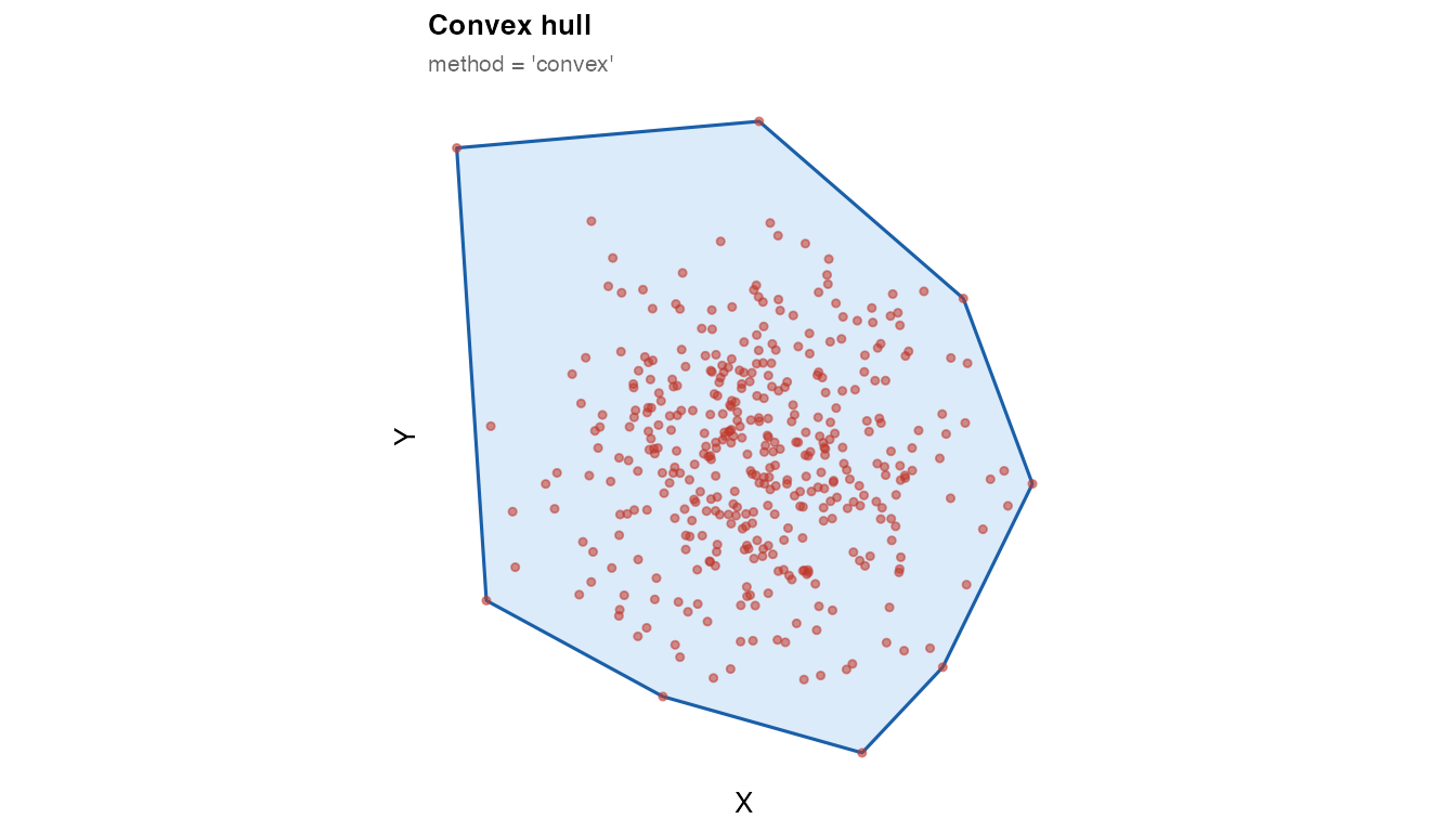

Use "convex" for quick sanity checks. For non-convex tissues — which is the norm in practice — use "concave" or "raster".

2. Concave hull

The concave hull wraps more tightly around the point cloud. The key parameter is concavity: lower values produce tighter, more concave boundaries; higher values approach the convex hull.

Requires the concaveman package.

# L-shaped cloud — non-convex; a good diagnostic
coords_L <- rbind(
  data.frame(x = runif(200, 0, 5), y = runif(200, 0, 1)),
  data.frame(x = runif(200, 0, 1), y = runif(200, 0, 5))
)

mask_convex_L  <- fit_spatial_mask(coords_L, method = "convex",
                                   verbose = FALSE)
mask_concave_L <- fit_spatial_mask(coords_L, method = "concave",
                                   concavity = 1.5, verbose = FALSE)

library(patchwork)
plot_mask(mask_convex_L, coords_L,
          title    = "Convex hull on L-shape",
          subtitle = "Incorrectly fills empty corner",
          fill = "#e74c3c", border = "#922b21") +
plot_mask(mask_concave_L, coords_L,
          title    = "Concave hull on L-shape (concavity = 1.5)",
          subtitle = "Correctly excludes the empty corner")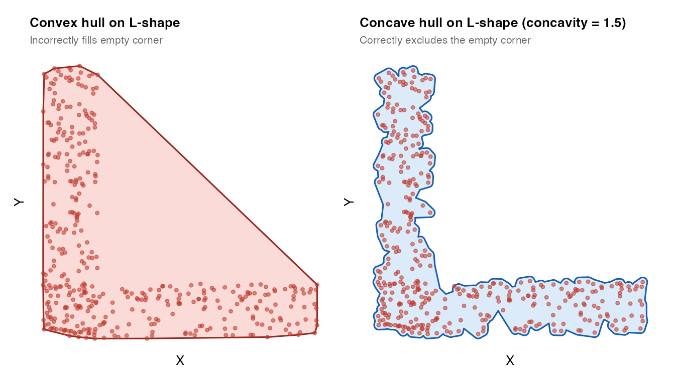

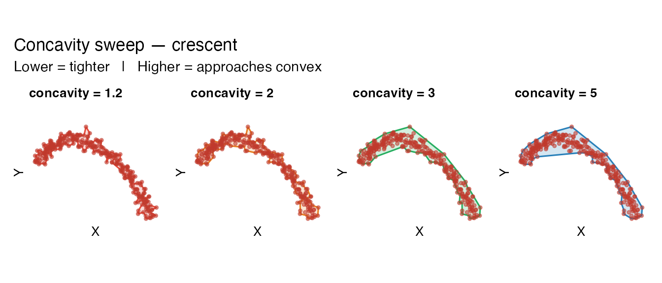
Concavity sweep

# Crescent-shaped cloud
theta <- seq(0.2, pi - 0.2, length.out = 300)
coords_cres <- data.frame(
  x = cos(theta) * (1 + rnorm(300, 0, 0.08)) * 3,
  y = sin(theta) * (1 + rnorm(300, 0, 0.08)) * 3 - cos(theta) * 1.5
)

pal <- c("#e74c3c", "#e67e22", "#27ae60", "#2980b9")
sw <- mapply(function(cv, col) {
  m <- fit_spatial_mask(coords_cres, method = "concave",
                        concavity = cv, verbose = FALSE)
  plot_mask(m, coords_cres, title = paste0("concavity = ", cv),
            fill = col, border = col)
}, c(1.2, 2, 3, 5), pal, SIMPLIFY = FALSE)

wrap_plots(sw, nrow = 1) +
  plot_annotation(
    title    = "Concavity sweep — crescent",
    subtitle = "Lower = tighter   |   Higher = approaches convex"
  )

3. KDE method

The KDE method estimates a 2-D kernel density surface and extracts a contour at a chosen probability level. It can represent holes and islands, but is slower for large datasets (n > 50,000). Requires MASS and isoband.

# Three-cluster cloud
mk_cluster <- function(n, cx, cy, sd = 0.4) {
  data.frame(x = rnorm(n, cx, sd), y = rnorm(n, cy, sd))
}
coords_multi <- rbind(mk_cluster(150, 0, 0), mk_cluster(150, 4, 1),
                      mk_cluster(150, 2, 4))

mask_kde_lo <- fit_spatial_mask(coords_multi, method = "kde",
                                 kde_threshold = 0.01, verbose = FALSE)
mask_kde_hi <- fit_spatial_mask(coords_multi, method = "kde",
                                 kde_threshold = 0.25, verbose = FALSE)

plot_mask(mask_kde_lo, coords_multi,
          title    = "KDE — low threshold (0.01)",
          subtitle = "One merged region",
          fill = "#27ae60", border = "#1e8449") +
plot_mask(mask_kde_hi, coords_multi,
          title    = "KDE — high threshold (0.25)",
          subtitle = "Separate masks per cluster",
          fill = "#8e44ad", border = "#6c3483")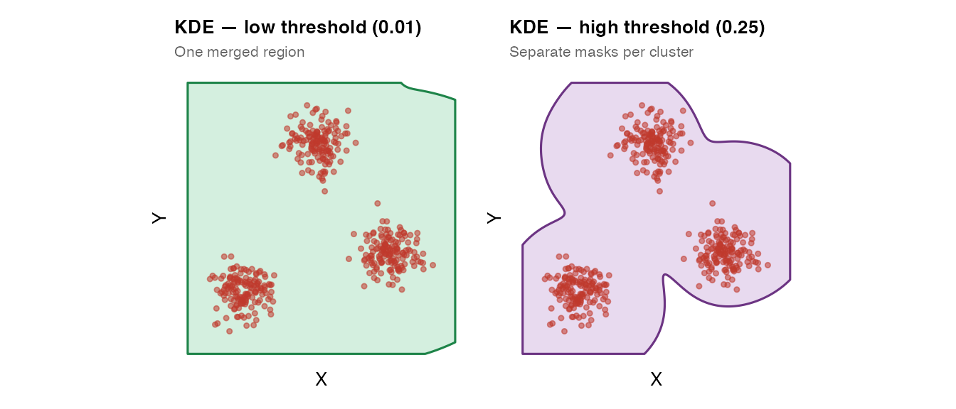

kde_threshold controls where the contour is drawn: - Lower values → larger mask (accepts sparse regions) - Higher values → smaller mask (only dense regions)

4. Raster method (recommended)

The raster method is the recommended default. It:

Bins point coordinates onto a regular grid.
Convolves the binary occupancy grid with a 2-D Gaussian of width raster_sigma (in coordinate units — the same units as x and y).
Thresholds at raster_threshold × max. Cells above threshold = “inside”.
Dissolves all “inside” cells via GEOS union. Holes and islands emerge automatically from the geometry — no ring-winding logic required.
Applies a morphological close to smooth the staircase boundary.

mask_raster <- fit_spatial_mask(coords_multi, method = "raster",
                                verbose = FALSE)
plot_mask(mask_raster, coords_multi,
          title    = "Raster method (default)",
          subtitle = "raster_sigma = NULL (auto = 3% of domain width)")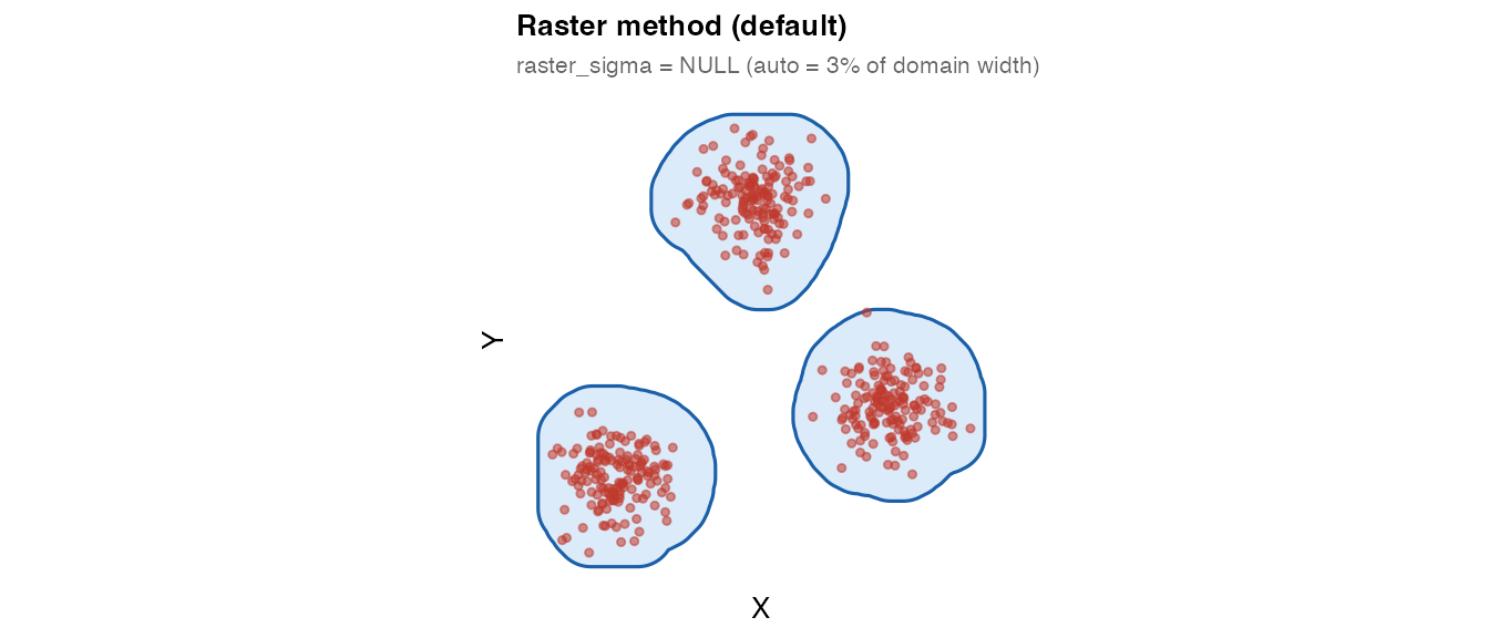

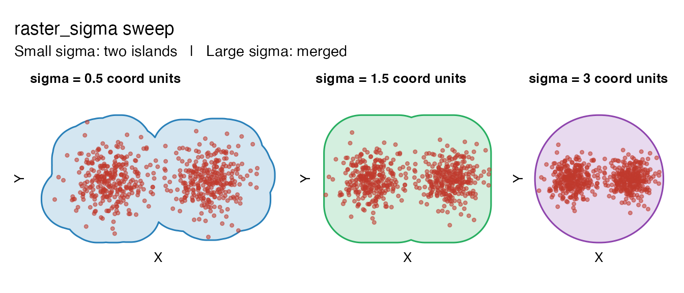
`raster_sigma` in coordinate units

The key innovation of the raster method is that raster_sigma is in coordinate units, not grid-cell units. This makes it directly interpretable: “how wide is the Gaussian around each point?”

# Two-cluster cloud with a gap
coords_gap <- rbind(
  data.frame(x = rnorm(300, 0, 1.5), y = rnorm(300, 0, 1.5)),
  data.frame(x = rnorm(300, 8, 1.5), y = rnorm(300, 0, 1.5))
)

sigmas <- c(0.5, 1.5, 3.0)
pal2   <- c("#2980b9", "#27ae60", "#8e44ad")
sw2 <- mapply(function(sig, col) {
  m <- fit_spatial_mask(coords_gap, method = "raster",
                        raster_sigma = sig, verbose = FALSE)
  plot_mask(m, coords_gap,
            title  = paste0("sigma = ", sig, " coord units"),
            fill   = col, border = col)
}, sigmas, pal2, SIMPLIFY = FALSE)

wrap_plots(sw2, nrow = 1) +
  plot_annotation(
    title    = "raster_sigma sweep",
    subtitle = "Small sigma: two islands   |   Large sigma: merged"
  )

5. Post-processing

Buffer expansion

buffer_dist expands the mask outward by a fixed distance after fitting. Useful when you want a small margin around the tissue edge.

mask_no_buf <- fit_spatial_mask(coords_circle, method = "raster",
                                buffer_dist = 0, verbose = FALSE)
mask_buf    <- fit_spatial_mask(coords_circle, method = "raster",
                                buffer_dist = 0.4, verbose = FALSE)

plot_mask(mask_no_buf, coords_circle,
          title = "No buffer (default)",
          subtitle = paste0("area = ",
                            round(as.numeric(sf::st_area(mask_no_buf)), 2))) +
plot_mask(mask_buf, coords_circle,
          title    = "buffer_dist = 0.4",
          subtitle = paste0("area = ",
                            round(as.numeric(sf::st_area(mask_buf)), 2)),
          fill = "#27ae60", border = "#1e8449")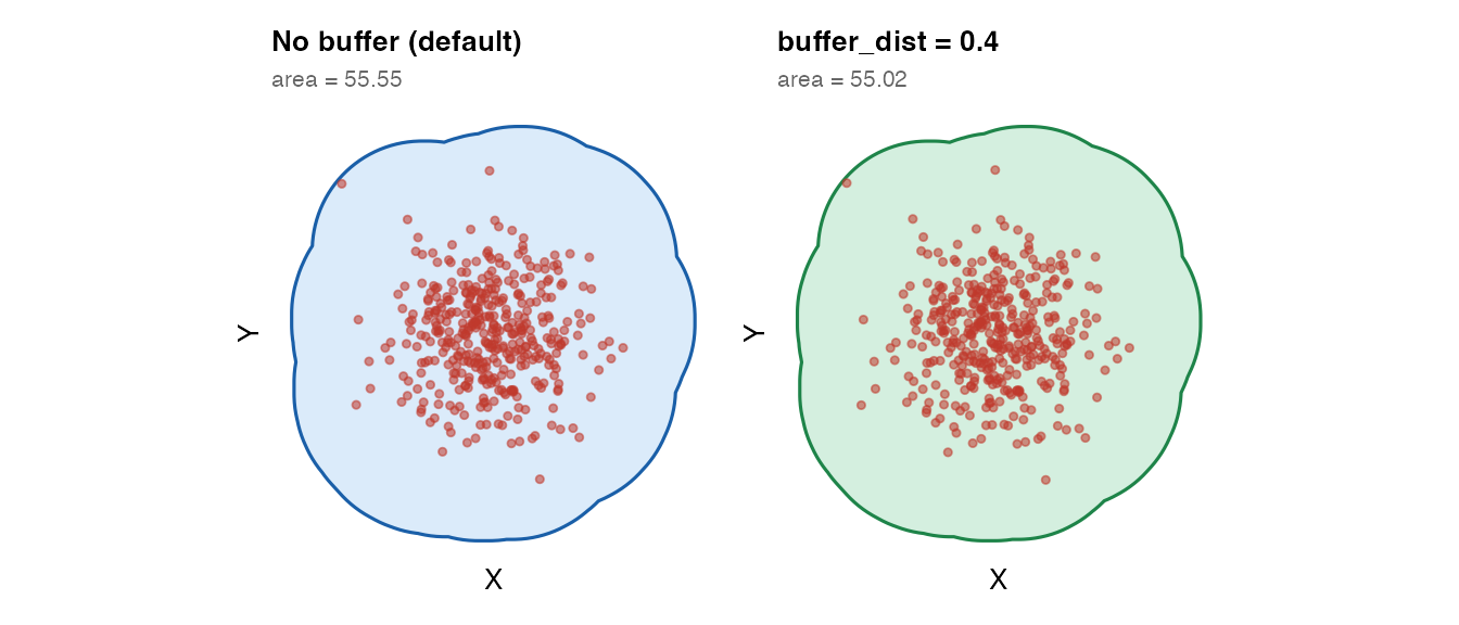

Boundary simplification

smooth_mask = TRUE applies Douglas–Peucker simplification to reduce vertex count while preserving overall shape.

mask_raw    <- fit_spatial_mask(coords_circle, method = "raster",
                                smooth_mask = FALSE, verbose = FALSE)
mask_smooth <- fit_spatial_mask(coords_circle, method = "raster",
                                smooth_mask = TRUE,
                                smooth_tolerance = 0.05, verbose = FALSE)

plot_mask(mask_raw, coords_circle,
          title = "No smoothing") +
plot_mask(mask_smooth, coords_circle,
          title    = "smooth_mask = TRUE (tolerance = 0.05)",
          fill = "#8e44ad", border = "#6c3483")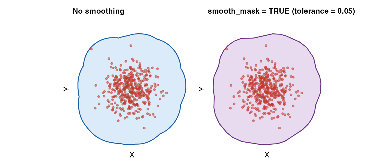

6. Verifying point containment

fit_spatial_mask() includes a built-in containment guarantee: after fitting, all input points are checked against the mask and a corrective buffer is applied if any fall outside. You can verify this explicitly:

coords_test <- data.frame(
  x = c(rnorm(300, 0, 3), rnorm(300, 12, 3)),
  y = c(rnorm(300, 0, 3), rnorm(300, 12, 3))
)
mask_test <- fit_spatial_mask(coords_test, method = "raster", verbose = FALSE)

pts_sfc   <- sf::st_as_sf(coords_test, coords = c("x", "y"),
                           crs = sf::NA_crs_)
# Use st_covered_by (not st_within): boundary points count as covered.
contained <- sf::st_covered_by(sf::st_geometry(pts_sfc),
                                sf::st_union(mask_test), sparse = FALSE)

cat("Points inside or on mask boundary:", sum(contained[, 1]),
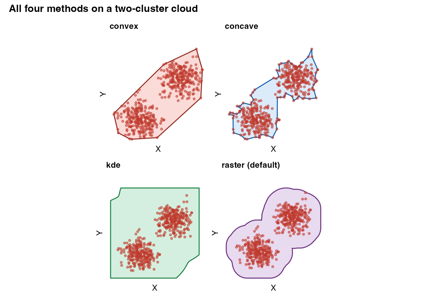
    "/", nrow(coords_test), "\n")

## Points inside or on mask boundary: 600 / 600

7. Method comparison

coords_demo <- rbind(
  data.frame(x = rnorm(250, 0, 2), y = rnorm(250, 0, 2)),
  data.frame(x = rnorm(250, 9, 2), y = rnorm(250, 9, 2))
)

m_cv <- fit_spatial_mask(coords_demo, method = "convex",  verbose = FALSE)
m_cc <- fit_spatial_mask(coords_demo, method = "concave", verbose = FALSE)
m_kd <- fit_spatial_mask(coords_demo, method = "kde",     verbose = FALSE)
m_ra <- fit_spatial_mask(coords_demo, method = "raster",  verbose = FALSE)

(plot_mask(m_cv, coords_demo, title = "convex",
           fill = "#e74c3c", border = "#922b21") +
 plot_mask(m_cc, coords_demo, title = "concave")) /
(plot_mask(m_kd, coords_demo, title = "kde",
           fill = "#27ae60", border = "#1e8449") +
 plot_mask(m_ra, coords_demo, title = "raster (default)",
           fill = "#8e44ad", border = "#6c3483")) +
plot_annotation(
  title = "All four methods on a two-cluster cloud",
  theme = theme(plot.title = element_text(face = "bold", size = 12))
)

Function reference summary

fit_spatial_mask(
  coords,

  # Method
  method            = "raster",   # "convex" | "concave" | "kde" | "raster"

  # Concave hull
  concavity         = 2,          # lower = tighter
  length_threshold  = 0,

  # KDE
  kde_bandwidth     = NULL,       # NULL = bandwidth.nrd auto
  kde_threshold     = 0.05,       # lower = larger mask
  kde_resolution    = 256L,

  # Raster
  raster_resolution = 256L,
  raster_sigma      = NULL,       # coordinate units; NULL = 3% of domain
  raster_threshold  = 0.15,       # lower = larger mask
  raster_min_pts    = 1L,

  # Post-processing
  buffer_dist       = 0,
  smooth_mask       = FALSE,
  smooth_tolerance  = NULL,

  # Misc
  n_cores           = 1L,
  crs               = NA,
  plot              = FALSE,
  verbose           = TRUE
)

Next steps

For topologically complex tissues (holes, islands), see the Holes, Islands, and Parameter Tuning vignette.
To estimate molecular concentration fields on a fitted mask, see the companion package TissueField.

Raredon Laboratory · Yale School of Medicine

2026-04-04

Why spatial masks?

Installation

Method overview

Shared plotting helper

1. Convex hull

2. Concave hull

Concavity sweep

3. KDE method

4. Raster method (recommended)

`raster_sigma` in coordinate units

5. Post-processing

Buffer expansion

Boundary simplification

6. Verifying point containment

7. Method comparison

Function reference summary

Next steps

Getting Started with TissueMask

Raredon Laboratory · Yale School of Medicine

2026-04-04

Why spatial masks?

Installation

Method overview

Shared plotting helper

1. Convex hull

2. Concave hull

Concavity sweep

3. KDE method

4. Raster method (recommended)

raster_sigma in coordinate units

5. Post-processing

Buffer expansion

Boundary simplification

6. Verifying point containment

7. Method comparison

Function reference summary

Next steps

`raster_sigma` in coordinate units