Holes, Islands, and Parameter Tuning

Overview

Real tissue architecture is topologically rich. Common features include:

Vessel lumens — circular or elliptical voids inside solid tissue
Necrotic cores — large central voids in tumour tissue
Tissue tears and processing artefacts — irregular internal gaps
Disconnected fragments — multiple separate tissue pieces on the same slide

The "raster" method in fit_spatial_mask() handles all of these naturally: by dissolving above-threshold grid cells via GEOS union, holes and islands emerge automatically from the geometry with no special-case logic. This vignette demonstrates each topology type and shows how to tune the two key parameters — raster_sigma and raster_threshold — to control the result.

library(TissueMask)
library(sf)
library(ggplot2)
library(patchwork)

set.seed(123)

1. Donut: single interior hole

The simplest topological case is a ring-shaped tissue — e.g., a cross-section through a vessel wall. Points are concentrated in an annulus; the centre is empty.

# Points uniformly distributed in an annulus (inner r=2, outer r=5)
r_d          <- sqrt(runif(800, 2^2, 5^2))
th_d         <- runif(800, 0, 2 * pi)
coords_donut <- data.frame(x = r_d * cos(th_d), y = r_d * sin(th_d))

# Raster: hole emerges automatically
mask_donut_raster <- fit_spatial_mask(coords_donut, method = "raster",
  raster_sigma = 0.25, raster_threshold = 0.2, verbose = FALSE)

# Convex hull: fills the hole
mask_donut_convex <- fit_spatial_mask(coords_donut, method = "convex",
                                      verbose = FALSE)

plot_mask(mask_donut_raster, coords_donut,
          title    = "Raster — hole detected",
          subtitle = paste0("sigma = 0.25 coord units  |  threshold = 0.2  |  ",
                            length(sf::st_cast(mask_donut_raster, "POLYGON")),
                            " polygon(s)")) +
plot_mask(mask_donut_convex, coords_donut,
          title    = "Convex hull — hole filled",
          subtitle = "method = 'convex' cannot represent holes",
          fill = "#e74c3c", border = "#922b21") +
plot_annotation(
  title = "Donut: vessel lumen topology",
  theme = theme(plot.title = element_text(face = "bold", size = 12))
)

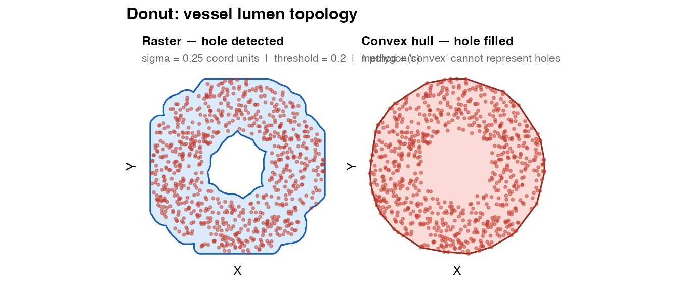
The raster mask is a POLYGON with one interior ring (hole). The convex hull is a solid disc — it cannot represent the void.

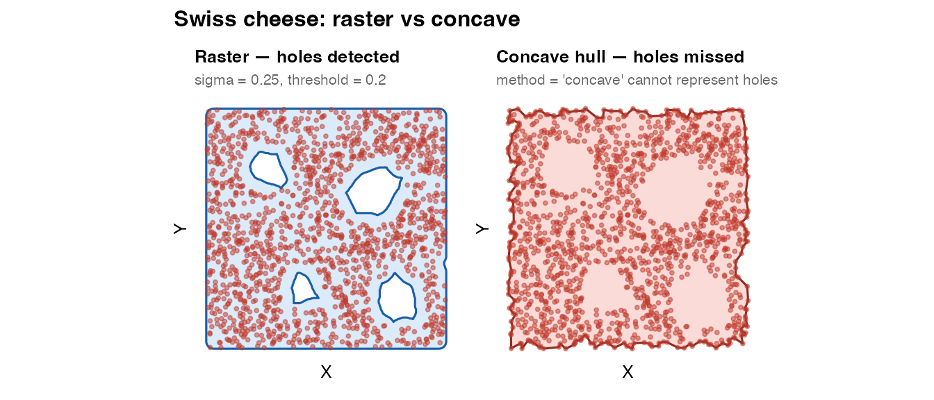
2. Swiss cheese: multiple holes

A square tissue block with four circular voids — representative of tissue with multiple vessel lumens or punch artefacts.

# Build ground-truth region: 10x10 square minus four circles
hdefs <- list(
  list(cx = 2.5, cy = 7.5, r = 1.1),
  list(cx = 7.0, cy = 6.5, r = 1.4),
  list(cx = 4.0, cy = 2.5, r = 0.9),
  list(cx = 8.0, cy = 2.0, r = 1.2)
)
outer_sq <- sf::st_sfc(sf::st_polygon(list(
  rbind(c(0,0), c(10,0), c(10,10), c(0,10), c(0,0)))))
hcircles <- lapply(hdefs, function(h) {
  sf::st_polygon(list(.circle_mat(h$cx, h$cy, h$r)))
})
swiss_region  <- sf::st_difference(outer_sq,
                   sf::st_sfc(sf::st_union(sf::st_sfc(hcircles))))
coords_swiss  <- sample_in_polygon(swiss_region, n = 1500)

mask_swiss <- fit_spatial_mask(coords_swiss, method = "raster",
  raster_sigma = 0.25, raster_threshold = 0.2, verbose = FALSE)

plot_mask(mask_swiss, coords_swiss,
          title    = "Swiss cheese — raster method",
          subtitle = "10x10 square with four circular voids")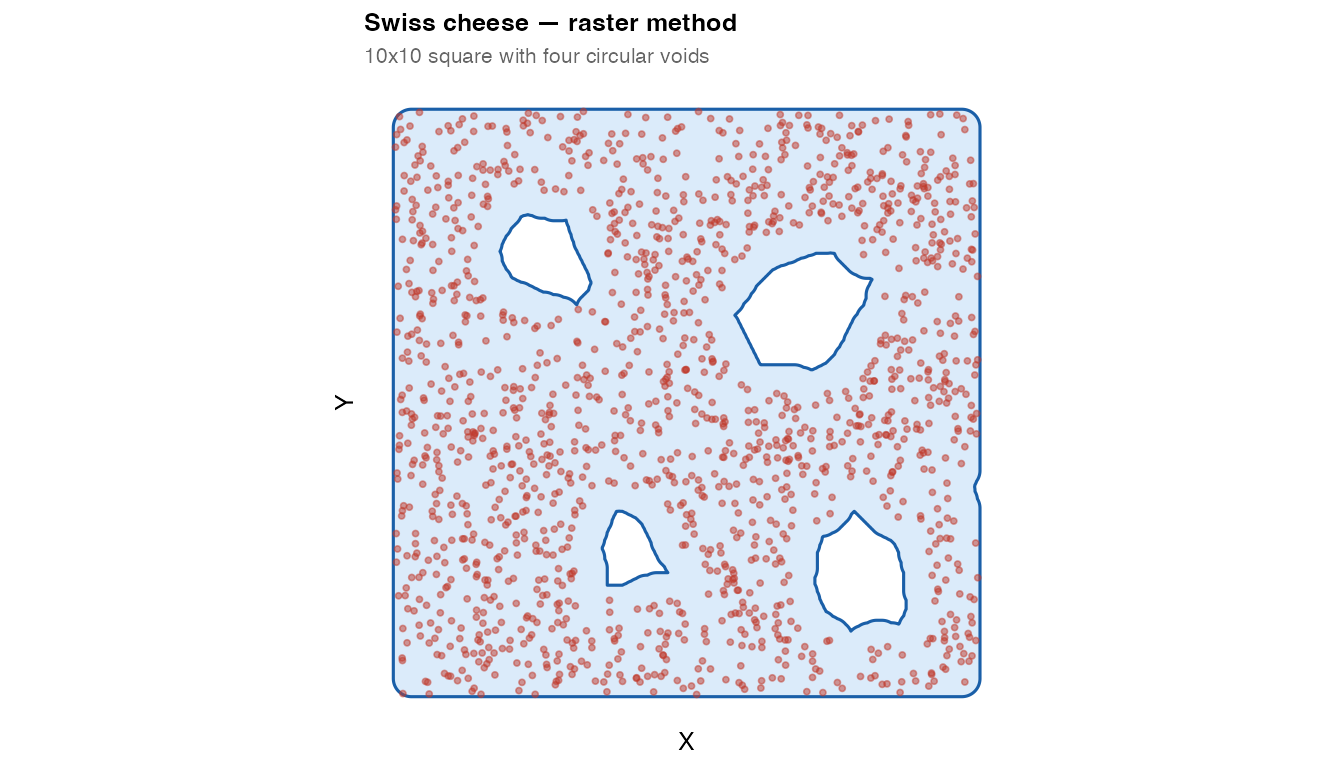

mask_swiss_concave <- fit_spatial_mask(coords_swiss, method = "concave",
                                        concavity = 1.8, verbose = FALSE)

plot_mask(mask_swiss, coords_swiss,
          title    = "Raster — holes detected",
          subtitle = "sigma = 0.25, threshold = 0.2") +
plot_mask(mask_swiss_concave, coords_swiss,
          title    = "Concave hull — holes missed",
          subtitle = "method = 'concave' cannot represent holes",
          fill = "#e74c3c", border = "#922b21") +
plot_annotation(
  title = "Swiss cheese: raster vs concave",
  theme = theme(plot.title = element_text(face = "bold", size = 12))
)

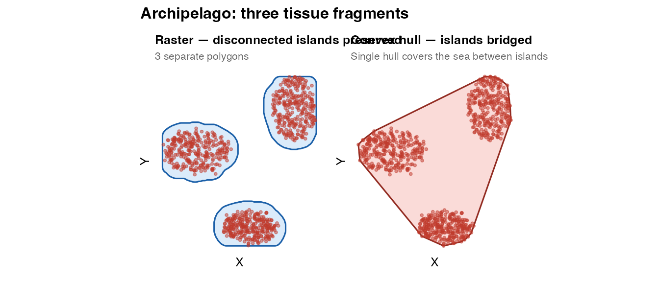
3. Archipelago: disconnected islands

Multiple disconnected tissue fragments — e.g., from sectioning — appear as separate spatial clusters. The raster method represents these as a MULTIPOLYGON, while a convex hull bridges them into one solid region.

mk_isl <- function(n, cx, cy, rx, ry, ns = 0.15) {
  th <- runif(n, 0, 2 * pi)
  r  <- sqrt(runif(n))
  data.frame(
    x = cx + r * rx * cos(th) + rnorm(n, 0, ns),
    y = cy + r * ry * sin(th) + rnorm(n, 0, ns)
  )
}
coords_arch <- rbind(
  mk_isl(300, 0,  0,  3, 2),
  mk_isl(300, 9,  4,  2, 3),
  mk_isl(300, 5, -7, 2.5, 1.5)
)

mask_arch_raster <- fit_spatial_mask(coords_arch, method = "raster",
  raster_sigma = 0.4, raster_threshold = 0.18, verbose = FALSE)
mask_arch_convex <- fit_spatial_mask(coords_arch, method = "convex",
                                      verbose = FALSE)

n_islands <- length(sf::st_cast(mask_arch_raster, "POLYGON"))

plot_mask(mask_arch_raster, coords_arch,
          title    = "Raster — disconnected islands preserved",
          subtitle = paste0(n_islands, " separate polygons")) +
plot_mask(mask_arch_convex, coords_arch,
          title    = "Convex hull — islands bridged",
          subtitle = "Single hull covers the sea between islands",
          fill = "#e74c3c", border = "#922b21") +
plot_annotation(
  title = "Archipelago: three tissue fragments",
  theme = theme(plot.title = element_text(face = "bold", size = 12))
)

4. `raster_sigma` sweep

raster_sigma is the most important tuning parameter. It controls the Gaussian spread applied to the occupancy grid in coordinate units (the same units as x and y). This makes it directly interpretable:

“How wide is the Gaussian around each point?”

Small raster_sigma → each point influences only its immediate neighbourhood → fine gaps and voids are preserved → risk of over-fragmentation
Large raster_sigma → points influence a larger area → voids fill in and islands merge → risk of over-merging

# Donut cloud — clear hole with adjustable fill behaviour
sigmas <- c(0.15, 0.3, 0.6, 1.0, 1.4, 1.7)
pal    <- c("#2c3e50", "#2980b9", "#27ae60",
            "#f39c12", "#e74c3c", "#8e44ad")

sw_plots <- mapply(function(sig, col) {
  m <- fit_spatial_mask(coords_donut, method = "raster",
                        raster_sigma = sig, raster_threshold = 0.2,
                        verbose = FALSE)
  n_poly <- length(sf::st_cast(m, "POLYGON"))
  plot_mask(m, coords_donut,
            title    = paste0("sigma = ", sig),
            subtitle = paste0(n_poly, " polygon(s)"),
            fill = col, border = col)
}, sigmas, pal, SIMPLIFY = FALSE)

wrap_plots(sw_plots, ncol = 3) +
  plot_annotation(
    title    = "raster_sigma sweep on donut cloud",
    subtitle = paste0("Small sigma: hole preserved   |   ",
                      "Large sigma: hole fills in"),
    theme = theme(
      plot.title    = element_text(face = "bold", size = 12),
      plot.subtitle = element_text(size = 9, color = "grey40")
    )
  )

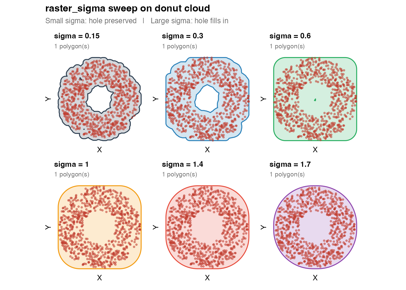
Interpretation: The hole is visible at sigma = 0.15 – 0.6. Around sigma = 1.0–1.4 it begins to fill. By sigma = 1.7 (roughly 17% of the domain width) the annulus has merged into a solid disc. Choose raster_sigma to be just larger than the typical inter-point gap, but smaller than the smallest void you want to preserve.

A useful heuristic: set raster_sigma to roughly 2–3× the typical nearest-neighbour distance in your point cloud.

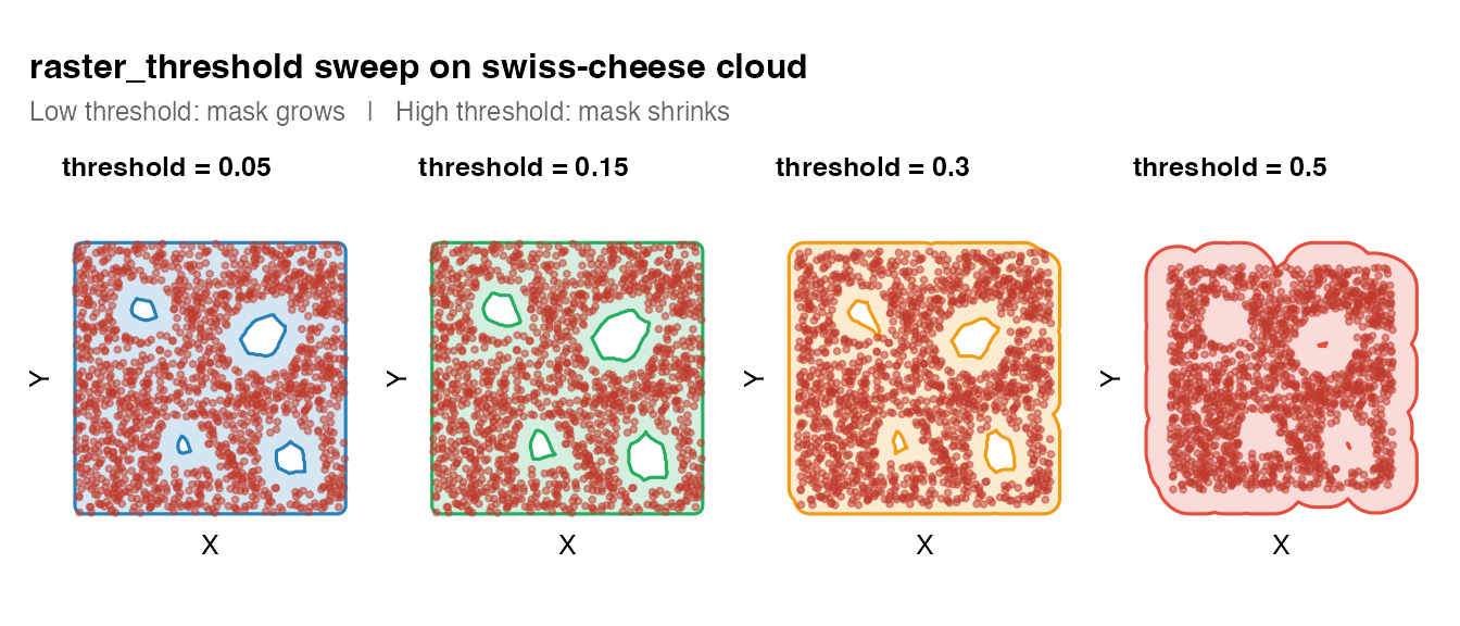
5. `raster_threshold` sweep

raster_threshold controls how the smoothed field is binarised: a cell is “inside” when its smoothed value exceeds raster_threshold × max. The effect is like adjusting the isocontour level on a density map.

thresholds <- c(0.05, 0.15, 0.30, 0.50)
pal_th     <- c("#2980b9", "#27ae60", "#f39c12", "#e74c3c")

th_plots <- mapply(function(thr, col) {
  m <- fit_spatial_mask(coords_swiss, method = "raster",
                        raster_sigma = 0.25, raster_threshold = thr,
                        verbose = FALSE)
  plot_mask(m, coords_swiss,
            title    = paste0("threshold = ", thr),
            fill = col, border = col)
}, thresholds, pal_th, SIMPLIFY = FALSE)

wrap_plots(th_plots, nrow = 1) +
  plot_annotation(
    title    = "raster_threshold sweep on swiss-cheese cloud",
    subtitle = "Low threshold: mask grows   |   High threshold: mask shrinks",
    theme = theme(
      plot.title    = element_text(face = "bold", size = 12),
      plot.subtitle = element_text(size = 9, color = "grey40")
    )
  )

6. Raster vs KDE — when to choose each

# Fractured-map cloud: irregular coast + multiple interior lakes
# (small n for vignette build speed)
th_f  <- seq(0, 2 * pi, length.out = 200)
r_c   <- 6 + 1.5 * sin(3 * th_f) + 0.8 * sin(7 * th_f)
mat_f <- cbind(r_c * cos(th_f), r_c * sin(th_f))
mat_f <- rbind(mat_f, mat_f[1L, ])
outer_coast <- sf::st_sfc(sf::st_polygon(list(mat_f)))

make_ellipse_poly <- function(cx, cy, a, b, angle_deg, n = 60) {
  th  <- seq(0, 2 * pi, length.out = n)
  ang <- angle_deg * pi / 180
  xe  <- a * cos(th); ye <- b * sin(th)
  mat <- cbind(cx + xe * cos(ang) - ye * sin(ang),
               cy + xe * sin(ang) + ye * cos(ang))
  mat <- rbind(mat, mat[1L, ])
  sf::st_polygon(list(mat))
}

lakes <- sf::st_sfc(list(
  make_ellipse_poly(-2.5,  3.0, 1.5, 0.8,  30),
  make_ellipse_poly( 3.5,  1.5, 1.2, 1.0, -20),
  make_ellipse_poly( 1.0, -3.5, 1.8, 0.6,  60)
))
frac_region  <- sf::st_difference(outer_coast, sf::st_union(lakes))
coords_frac  <- sample_in_polygon(frac_region, n = 1200)

mask_frac_raster <- fit_spatial_mask(coords_frac, method = "raster",
  raster_sigma = 0.5, raster_threshold = 0.18, verbose = FALSE)
mask_frac_kde    <- fit_spatial_mask(coords_frac, method = "kde",
  kde_resolution = 200L, kde_threshold = 0.01, verbose = FALSE)

plot_mask(mask_frac_raster, coords_frac,
          title    = "Raster",
          subtitle = "sigma = 0.5, threshold = 0.18") +
plot_mask(mask_frac_kde, coords_frac,
          title    = "KDE",
          subtitle = "kde_threshold = 0.01",
          fill = "#27ae60", border = "#1e8449") +
plot_annotation(
  title = "Irregular coast + three lake voids",
  theme = theme(plot.title = element_text(face = "bold", size = 12))
)

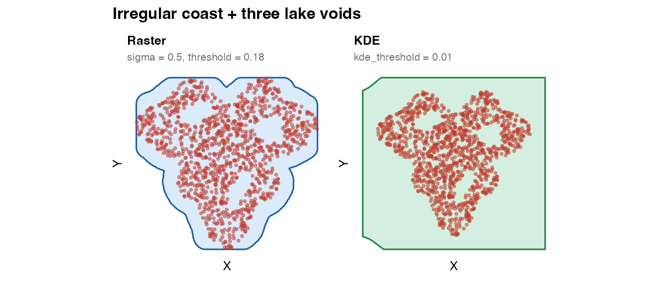
When to prefer raster: - Large point clouds (n > 50,000) — raster scales linearly; KDE is O(n²) - Datasets with sharp, well-defined tissue boundaries - When you want explicit raster_sigma control in interpretable units

When to prefer KDE: - Small to moderate n, dense and smooth point distributions - When bandwidth has a physical interpretation (e.g., cell radius) - When you have strongly anisotropic data and want anisotropic bandwidths

7. Scale and performance

The raster method is designed to scale to spatial transcriptomics datasets with tens or hundreds of thousands of molecules.

n points	raster (256×256)	kde (256×256)
1,000	< 0.1 s	< 0.1 s
10,000	~ 0.1 s	~ 0.5 s
100,000	~ 0.5 s	~ 60 s
1,000,000	~ 3 s	not recommended

Timings approximate; hardware-dependent. KDE scales with n via kde2d bandwidth estimation.

For very large datasets, increase raster_resolution (default 256) to 512 for finer boundaries, at roughly 4× the compute cost.

Parallel row-smoothing is available on Unix/macOS via n_cores > 1:

mask <- fit_spatial_mask(
  coords, method = "raster",
  raster_resolution = 512L,
  n_cores = 4L  # Unix/macOS only
)

Parameter tuning summary

Scenario	Recommended settings
Solid tissue, no voids	Any method; `"raster"` default is fine
Vessel lumens / necrotic cores	`"raster"`, `raster_sigma` ≈ 2–3× point spacing
Fine voids	`raster_sigma` small (0.1–0.3× void diameter)
Islands should merge	`raster_sigma` large (> gap width)
Mask too large	Increase `raster_threshold` (0.15 → 0.3)
Mask too small	Decrease `raster_threshold` (0.15 → 0.05)
Add margin around tissue	`buffer_dist > 0`
Reduce vertex count	`smooth_mask = TRUE`

Raredon Laboratory · Yale School of Medicine

2026-04-04

Overview

1. Donut: single interior hole

2. Swiss cheese: multiple holes

3. Archipelago: disconnected islands

4. `raster_sigma` sweep

5. `raster_threshold` sweep

6. Raster vs KDE — when to choose each

7. Scale and performance

Parameter tuning summary

Holes, Islands, and Parameter Tuning

Raredon Laboratory · Yale School of Medicine

2026-04-04

Overview

1. Donut: single interior hole

2. Swiss cheese: multiple holes

3. Archipelago: disconnected islands

4. raster_sigma sweep

5. raster_threshold sweep

6. Raster vs KDE — when to choose each

7. Scale and performance

Parameter tuning summary

4. `raster_sigma` sweep

5. `raster_threshold` sweep