Complete Reference: fit_spatial_mask()

Overview

In spatial transcriptomics and spatial proteomics experiments, the tissue of interest occupies some irregular region of a slide. Before computing any spatially-resolved quantity (cell-type composition, signaling gradients, niche structure), you need a reliable spatial mask: a polygon or multi-polygon that faithfully represents the shape of the tissue, including internal voids (vessel lumens, necrotic cores, tissue tears) and disconnected fragments.

fit_spatial_mask() takes a set of XY point coordinates — typically cell centroids or transcript locations — and fits a mask polygon to them. It supports four methods of increasing complexity:

Method	Topology	Speed	Best for
`"convex"`	No holes, no islands	Instant	Quick sanity checks
`"concave"`	No holes, no islands	Fast	Simple non-convex shapes
`"kde"`	Holes and islands	Moderate	Dense, smooth datasets
`"raster"`	Holes and islands	Fast at scale	Most use cases; recommended default

Setup

library(TissueMask)
library(sf)
library(ggplot2)
library(patchwork)

set.seed(42)

Shared plotting helper

Throughout this vignette we use a single plot_mask() helper. The key implementation note is that it uses geom_sf() rather than geom_polygon(). This is essential: geom_polygon() draws a line between the last vertex of the exterior ring and the first vertex of each interior (hole) ring, producing diagonal artefacts. geom_sf() delegates rendering to the sf/GEOS layer which handles holes correctly.

plot_mask <- function(mask, coords, title = "", subtitle = "",
                      fill = "#4c9be8", border = "#1a5fa8",
                      pt_col = "#c0392b", pt_size = 1.2, pt_alpha = 0.55) {
  mask_sf <- sf::st_sf(geometry = mask)
  ggplot() +
    geom_sf(data = mask_sf, fill = fill, alpha = 0.2,
            color = border, linewidth = 0.55) +
    geom_point(data = coords, aes(x = x, y = y),
               color = pt_col, size = pt_size, alpha = pt_alpha) +
    coord_sf(datum = NA) +
    labs(title = title, subtitle = subtitle, x = "X", y = "Y") +
    theme_minimal(base_size = 9.5) +
    theme(plot.title    = element_text(face = "bold", size = 9.5),
          plot.subtitle = element_text(size = 8, color = "grey40"),
          panel.grid    = element_line(color = "grey93"))
}

Function reference: `fit_spatial_mask()`

fit_spatial_mask(
  coords,

  # Method selection
  method            = "raster",   # "convex" | "concave" | "kde" | "raster"

  # Concave hull
  concavity         = 2,          # lower = tighter; higher = approaches convex
  length_threshold  = 0,

  # KDE
  kde_bandwidth     = NULL,       # NULL = auto (bandwidth.nrd)
  kde_threshold     = 0.05,       # quantile of density to threshold at
  kde_resolution    = 256L,

  # Raster (recommended)
  raster_resolution = 256L,       # grid cells per axis
  raster_sigma      = NULL,       # Gaussian spread in COORDINATE UNITS; NULL = 3% of domain
  raster_threshold  = 0.15,       # fraction of peak Gaussian field to threshold at
  raster_min_pts    = 1L,         # min points per cell to count as occupied

  # Post-processing
  buffer_dist       = 0,          # expand mask outward by this distance
  smooth_mask       = FALSE,      # simplify boundary (st_simplify)
  smooth_tolerance  = NULL,       # NULL = 1% of bounding box diagonal

  # Misc
  n_cores           = 1L,
  crs               = NA,
  plot              = FALSE,
  verbose           = TRUE
)

Return value

fit_spatial_mask() returns an sfc geometry object (the sf package’s geometry column class). You can:

Pass it directly to estimate_concentration_field() as the mask argument
Plot it with geom_sf()
Compute area with sf::st_area()
Test point containment with sf::st_covered_by()
Convert to a data frame with as.data.frame(sf::st_coordinates(mask))

Section 1 — Circular cloud: sanity check

The simplest possible test: a Gaussian cloud with no special topology. All three non-trivial methods should return similar results here. This section establishes that the function runs and that the three main methods agree on simple inputs.

n             <- 400
coords_circle <- data.frame(x = rnorm(n, 0, 1),
                             y = rnorm(n, 0, 1))

m1a <- fit_spatial_mask(coords_circle, method = "convex",  verbose = FALSE)
m1b <- fit_spatial_mask(coords_circle, method = "concave", concavity = 2,
                        verbose = FALSE)
m1c <- fit_spatial_mask(coords_circle, method = "kde",
                        kde_threshold = 0.02, buffer_dist = 0.1,
                        verbose = FALSE)

plot_mask(m1a, coords_circle, title = "1a. Convex hull",
          subtitle = "method='convex'") +
plot_mask(m1b, coords_circle, title = "1b. Concave hull",
          subtitle = "concavity=2") +
plot_mask(m1c, coords_circle, title = "1c. KDE contour",
          subtitle = "kde_threshold=0.02, buffer=0.1",
          fill = "#27ae60", border = "#1e8449") +
plot_annotation(
  title = "Section 1: Circular Cloud -- Sanity Check",
  theme = theme(plot.title = element_text(face = "bold", size = 13)))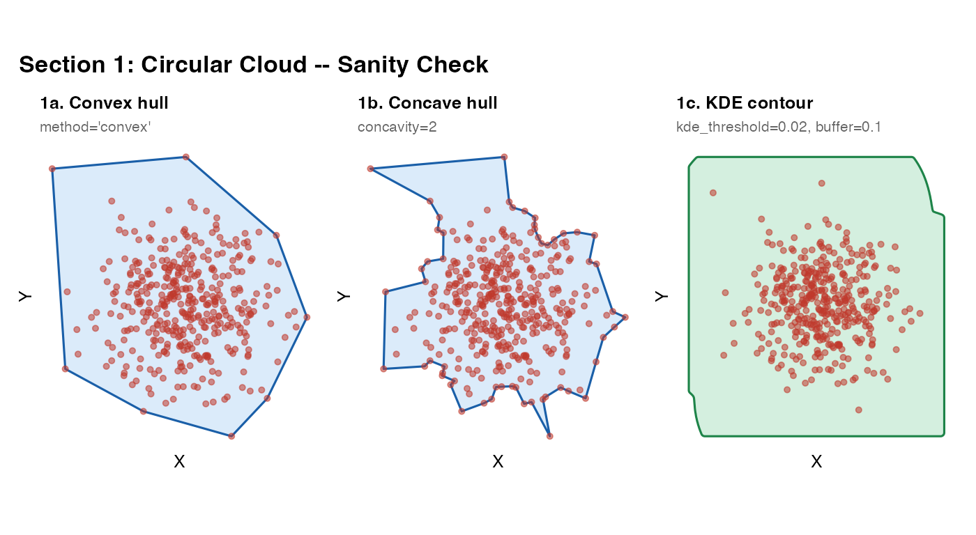

What to look for: All three masks should closely envelope the point cloud. Small differences near the boundary are expected – convex gives a polygon, KDE gives a smoother contour. Any large discrepancy here indicates a parameter problem.

Section 2 – Elongated cloud: anisotropy

Elongated tissue (e.g. a muscle section, a linear airway epithelium) has very different extents along its two axes. All methods should handle this naturally; this section confirms that no method is implicitly assuming isotropy.

coords_elong <- data.frame(x = rnorm(n, 0, 3),
                            y = rnorm(n, 0, 0.6))

m2a <- fit_spatial_mask(coords_elong, method = "convex",  verbose = FALSE)
m2b <- fit_spatial_mask(coords_elong, method = "concave", verbose = FALSE)
m2c <- fit_spatial_mask(coords_elong, method = "kde",
                        kde_threshold = 0.02, buffer_dist = 0.1,
                        verbose = FALSE)

plot_mask(m2a, coords_elong, title = "2a. Convex") +
plot_mask(m2b, coords_elong, title = "2b. Concave") +
plot_mask(m2c, coords_elong, title = "2c. KDE",
          fill = "#27ae60", border = "#1e8449") +
plot_annotation(
  title = "Section 2: Elongated Cloud",
  theme = theme(plot.title = element_text(face = "bold", size = 13)))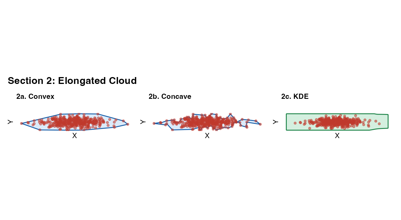

What to look for: The mask should track the long axis of the cloud, not default to a circle. The KDE bandwidth is computed separately for x and y (MASS::bandwidth.nrd), so it adapts to anisotropy automatically.

Section 3 – L-shaped cloud: the non-convex diagnostic

This is the most important basic test. The L-shape is the canonical non-convex case: the convex hull incorrectly fills the concave corner of the L, including empty space that contains no tissue. A good mask must track the actual boundary and exclude the corner.

Rule of thumb: If your tissue has any re-entrant angles (C-shapes, crescents, airways, arcs), do not use method = "convex". Use method = "concave" or method = "raster".

coords_L <- rbind(
  data.frame(x = runif(200, 0, 5) + rnorm(200, 0, 0.05),
             y = runif(200, 0, 1) + rnorm(200, 0, 0.05)),   # horizontal bar
  data.frame(x = runif(200, 0, 1) + rnorm(200, 0, 0.05),
             y = runif(200, 0, 5) + rnorm(200, 0, 0.05)))   # vertical bar

m3a <- fit_spatial_mask(coords_L, method = "convex",  verbose = FALSE)
m3b <- fit_spatial_mask(coords_L, method = "concave", concavity = 1.5, verbose = FALSE)
m3c <- fit_spatial_mask(coords_L, method = "concave", concavity = 3.0, verbose = FALSE)

plot_mask(m3a, coords_L,
          title    = "3a. Convex hull",
          subtitle = "Incorrectly includes empty corner",
          fill = "#e74c3c", border = "#922b21") +
plot_mask(m3b, coords_L,
          title    = "3b. Concave, tight (1.5)",
          subtitle = "Correctly excludes corner") +
plot_mask(m3c, coords_L,
          title    = "3c. Concave, relaxed (3.0)",
          subtitle = "Partially includes corner",
          fill = "#8e44ad", border = "#6c3483") +
plot_annotation(
  title    = "Section 3: L-Shaped Cloud -- Non-Convex",
  subtitle = "Lower concavity wraps more tightly; convex hull fails",
  theme    = theme(plot.title    = element_text(face = "bold", size = 13),
                   plot.subtitle = element_text(size = 9, color = "grey40")))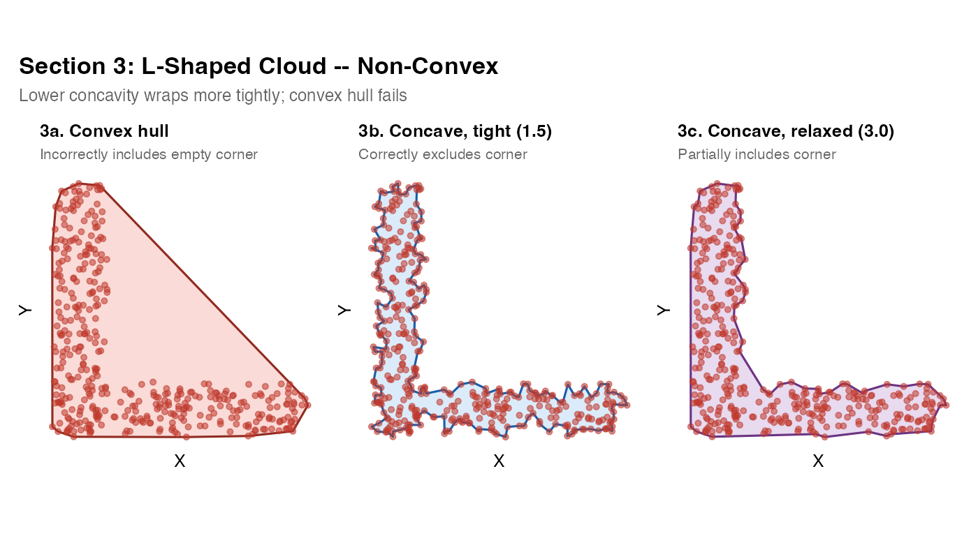

The `concavity` parameter

concavity controls how aggressively the hull “cuts in” to follow the data boundary. It is the key tuning parameter for method = "concave".

Value	Behaviour
1.0–1.5	Very tight – tracks the data boundary closely
2.0	Default – good balance for most tissue shapes
3.0–5.0	Relaxed – approaches the convex hull

When to use lower values: C-shapes, crescents, U-shapes, any tissue with a notch or bay. When to use higher values: Dense blobs where you want a smooth, padded boundary. If you see the mask cutting through the interior of your tissue, increase concavity. If it fills in empty space at concavities, decrease it.

Section 4 – Multi-cluster blobs: connected vs. isolated masks

When tissue fragments are well-separated, a low kde_threshold will produce a single mask that bridges them (because the KDE density never drops to zero between clusters at low thresholds). A higher threshold separates them into distinct polygons.

The raster method’s raster_sigma plays the analogous role: a large sigma bridges clusters; a small sigma isolates them.

mk_cluster <- function(n, cx, cy, sd = 0.4)
  data.frame(x = rnorm(n, cx, sd), y = rnorm(n, cy, sd))

coords_multi <- rbind(mk_cluster(150, 0, 0),
                      mk_cluster(150, 4, 1),
                      mk_cluster(150, 2, 4))

m4a <- fit_spatial_mask(coords_multi, method = "convex",  verbose = FALSE)
m4b <- fit_spatial_mask(coords_multi, method = "concave", concavity = 2,
                        verbose = FALSE)
m4c <- fit_spatial_mask(coords_multi, method = "kde",
                        kde_threshold = 0.01, buffer_dist = 0.15,
                        verbose = FALSE)
m4d <- fit_spatial_mask(coords_multi, method = "kde",
                        kde_threshold = 0.25, buffer_dist = 0.15,
                        verbose = FALSE)

(plot_mask(m4a, coords_multi, title = "4a. Convex") +
 plot_mask(m4b, coords_multi, title = "4b. Concave")) /
(plot_mask(m4c, coords_multi,
           title    = "4c. KDE -- inclusive",
           subtitle = "threshold=0.01: merged",
           fill = "#27ae60", border = "#1e8449") +
 plot_mask(m4d, coords_multi,
           title    = "4d. KDE -- tight",
           subtitle = "threshold=0.25: separated",
           fill = "#8e44ad", border = "#6c3483")) +
plot_annotation(
  title = "Section 4: Multi-Cluster",
  theme = theme(plot.title = element_text(face = "bold", size = 13)))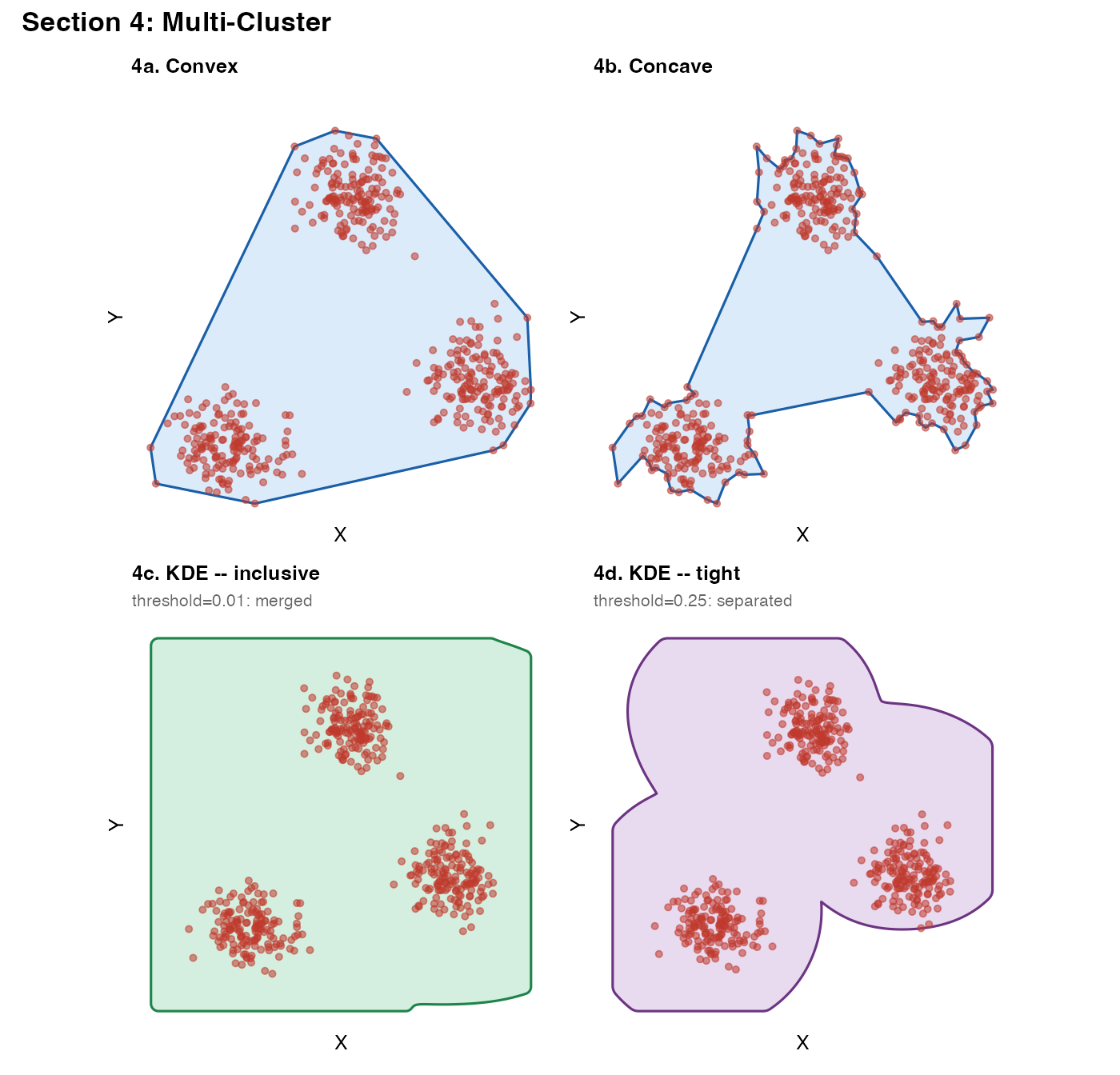

Choosing `kde_threshold`

kde_threshold is expressed as a quantile of the KDE density values across the grid.

Low values (0.01–0.05): the contour is drawn far out in the low-density tails. Clusters merge; mask is generous.
High values (0.15–0.30): only the dense core is enclosed. Clusters separate; mask is tight.

Practical advice: Start at 0.05 and increase until the mask matches your visual inspection. If you expect biologically separated regions (e.g. two lobes), a threshold that separates them is usually correct.

Section 5 – Concavity sweep on a crescent

A crescent is a severe test of the concave hull: it has a large, deep concavity spanning most of the shape. This sweep lets you calibrate the concavity parameter on a shape where the expected correct answer is obvious.

theta       <- seq(0.2, pi - 0.2, length.out = 300)
coords_cres <- data.frame(
  x = cos(theta) * (1 + rnorm(300, 0, 0.08)) * 3,
  y = sin(theta) * (1 + rnorm(300, 0, 0.08)) * 3 - cos(theta) * 1.5)

pal <- c("#e74c3c", "#e67e22", "#27ae60", "#2980b9")
sw  <- mapply(function(cv, col) {
  m <- fit_spatial_mask(coords_cres, method = "concave",
                        concavity = cv, verbose = FALSE)
  plot_mask(m, coords_cres, title = paste0("concavity = ", cv),
            fill = col, border = col)
}, c(1.2, 2, 3, 5), pal, SIMPLIFY = FALSE)

wrap_plots(sw, nrow = 1) +
  plot_annotation(
    title    = "Section 5: Concavity Sweep -- Crescent",
    subtitle = "Lower = tighter | Higher = approaches convex hull",
    theme    = theme(plot.title    = element_text(face = "bold", size = 13),
                     plot.subtitle = element_text(size = 9, color = "grey40")))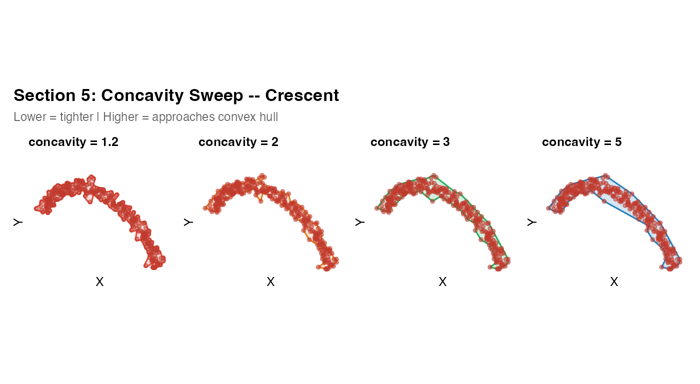

What to look for: At concavity = 1.2, the hull cuts tightly around the arc. At concavity = 5, it is nearly convex and fills the interior. The “correct” value for real tissue is the one that matches a human drawing of the tissue boundary. For a crescent-shaped airway section, 1.2--1.5 is usually appropriate.

Section 6 – Buffer and smoothing

After fitting, two post-processing options are available:

buffer_dist: expands the mask outward by this distance in coordinate units using sf::st_buffer(). Useful when you want a small safety margin to ensure all cells fall inside the mask, or when points are sparse near the boundary.
smooth_mask: applies sf::st_simplify() to reduce the vertex count and round jagged boundary segments. Controlled by smooth_tolerance (default: 1% of bounding box diagonal).

r           <- sqrt(runif(250, 0.4^2, 1^2))
ang         <- runif(250, 0, 2 * pi)
coords_ring <- data.frame(x = r * cos(ang) * 5,
                           y = r * sin(ang) * 5)

m6a <- fit_spatial_mask(coords_ring, method = "concave", concavity = 2,
                        buffer_dist = 0,   smooth_mask = FALSE, verbose = FALSE)
m6b <- fit_spatial_mask(coords_ring, method = "concave", concavity = 2,
                        buffer_dist = 0.3, smooth_mask = FALSE, verbose = FALSE)
m6c <- fit_spatial_mask(coords_ring, method = "concave", concavity = 2,
                        buffer_dist = 0.3, smooth_mask = TRUE,
                        smooth_tolerance = 0.15, verbose = FALSE)

plot_mask(m6a, coords_ring,
          title = "6a. Raw -- no buffer, no smooth") +
plot_mask(m6b, coords_ring,
          title = "6b. Buffer = 0.3",
          fill = "#27ae60", border = "#1e8449") +
plot_mask(m6c, coords_ring,
          title = "6c. Buffer + smooth",
          subtitle = "smooth_tolerance = 0.15",
          fill = "#8e44ad", border = "#6c3483") +
plot_annotation(
  title = "Section 6: Buffer and Smoothing",
  theme = theme(plot.title = element_text(face = "bold", size = 13)))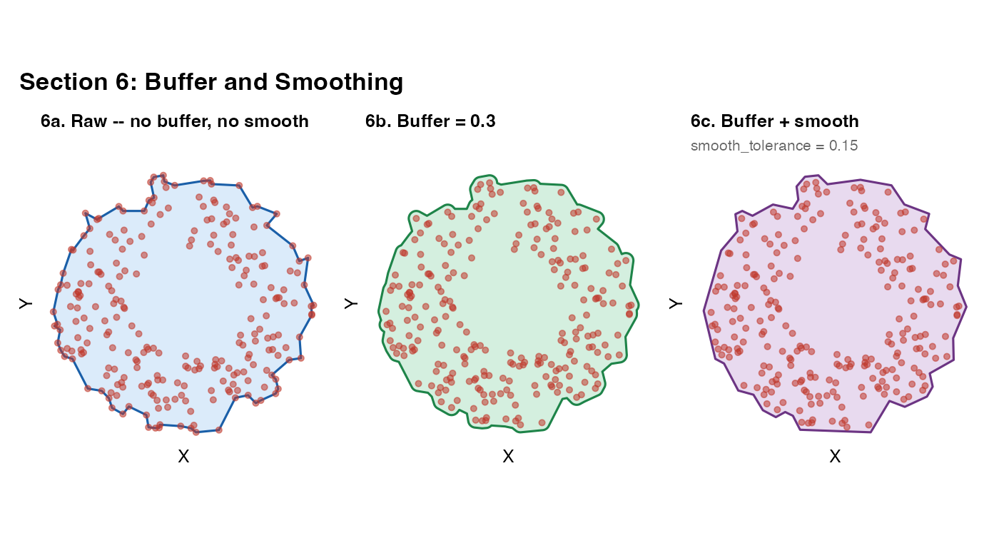

When to use each:

buffer_dist: use when downstream point-in-mask tests are failing for points you know should be inside (e.g. points right on the boundary). A value of 1–5% of the domain width is usually safe.
smooth_mask: use when you want a visually clean boundary for publication figures, or when a jagged boundary is causing downstream geometric operations to be slow or numerically unstable. Be careful: large smooth_tolerance values can erase real tissue features.

Section 7 – Topologically complex cases: holes and islands

The "raster" method is the recommended approach for masks that need to represent holes (vessel lumens, necrotic cores, tissue tears) or disconnected islands. It is also the fastest method for large point clouds (100k+ cells).

How the raster method works

Bin all points onto a regular raster_resolution x raster_resolution grid.
Convolve the binary occupancy grid with a 2D isotropic Gaussian of width raster_sigma (in coordinate units). This is equivalent to placing a Gaussian “blob” at every point and summing – the value at each cell represents how much point density is nearby.
Threshold at raster_threshold x max(field). Cells above threshold are “inside”; cells below are “outside”.
Build one axis-aligned rectangle per inside cell, then dissolve all rectangles with sf::st_union(). GEOS handles the topology automatically – holes and islands emerge from the geometry without any ring-winding logic.
Smooth the staircase boundary with a morphological close (buffer out then in by ~half the cell diagonal).

Key tuning parameters

Parameter	Effect
`raster_sigma` (larger)	Holes fill in, islands merge, boundary smooths
`raster_sigma` (smaller)	Fine holes and gaps preserved
`raster_threshold` (larger)	Mask shrinks; requires denser local coverage
`raster_threshold` (smaller)	Mask grows; accepts sparse regions
`raster_resolution` (larger)	Finer grid; more detail; slower union step

Units note: raster_sigma is in coordinate units (same as x and y). If your tissue coordinates span 0–10, a raster_sigma of 0.25 means each Gaussian blob has a standard deviation of 0.25 tissue units. NULL sets sigma automatically to 3% of the domain width.

7a – Donut: single interior void

r_d          <- sqrt(runif(800, 2^2, 5^2))
th_d         <- runif(800, 0, 2 * pi)
coords_donut <- data.frame(x = r_d * cos(th_d),
                            y = r_d * sin(th_d))

m7a_r <- fit_spatial_mask(coords_donut, method = "raster",
  raster_resolution = 256L, raster_sigma = 0.25, raster_threshold = 0.2,
  verbose = FALSE)
m7a_c <- fit_spatial_mask(coords_donut, method = "convex", verbose = FALSE)

plot_mask(m7a_r, coords_donut,
          title    = "7a-i. Raster -- hole detected",
          subtitle = "sigma = 0.25 coord units, threshold = 0.2") +
plot_mask(m7a_c, coords_donut,
          title    = "7a-ii. Convex -- hole filled",
          subtitle = "Convex hull cannot represent holes",
          fill = "#e74c3c", border = "#922b21") +
plot_annotation(
  title = "Donut: Single Interior Void",
  theme = theme(plot.title = element_text(face = "bold", size = 13)))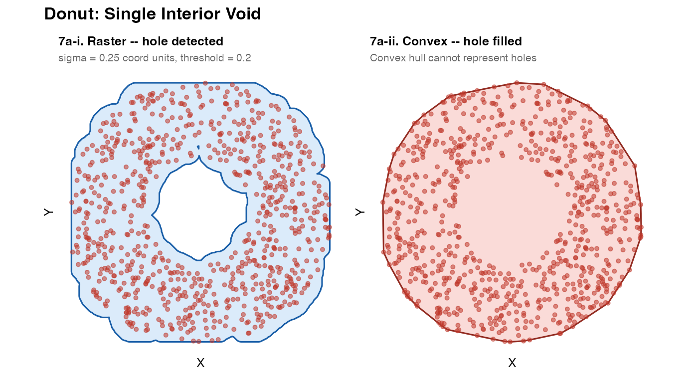

The raster method naturally detects the empty centre as a region of low convolved density, below the threshold. The convex hull cannot ever represent a hole – it is by definition the smallest convex polygon containing all the points.

7b – Swiss cheese: multiple holes

.circle_mat <- function(cx, cy, r, n = 100) {
  th  <- seq(0, 2 * pi, length.out = n)
  mat <- cbind(cx + r * cos(th), cy + r * sin(th))
  rbind(mat, mat[1L, ])
}

hdefs <- list(
  list(cx = 2.5, cy = 7.5, r = 1.1),
  list(cx = 7.0, cy = 6.5, r = 1.4),
  list(cx = 4.0, cy = 2.5, r = 0.9),
  list(cx = 8.0, cy = 2.0, r = 1.2)
)

sample_in_polygon <- function(poly_sf, n, max_tries = 20) {
  bb <- sf::st_bbox(poly_sf)
  mu <- sf::st_union(poly_sf)
  pts <- data.frame(x = numeric(0), y = numeric(0))
  for (i in seq_len(max_tries)) {
    if (nrow(pts) >= n) break
    cnd <- data.frame(x = runif(n * 8, bb["xmin"], bb["xmax"]),
                      y = runif(n * 8, bb["ymin"], bb["ymax"]))
    ok  <- as.logical(sf::st_within(
      sf::st_as_sf(cnd, coords = c("x","y")), mu, sparse = FALSE)[, 1L])
    pts <- rbind(pts, cnd[ok, ])
  }
  pts[seq_len(min(n, nrow(pts))), ]
}

outer_sq     <- sf::st_sfc(sf::st_polygon(list(
  rbind(c(0,0), c(10,0), c(10,10), c(0,10), c(0,0)))))
hcircles     <- lapply(hdefs, function(h)
  sf::st_polygon(list(.circle_mat(h$cx, h$cy, h$r))))
swiss_region <- sf::st_difference(outer_sq,
  sf::st_sfc(sf::st_union(sf::st_sfc(hcircles))))
coords_swiss <- sample_in_polygon(swiss_region, n = 1500)

m7b_r <- fit_spatial_mask(coords_swiss, method = "raster",
  raster_resolution = 256L, raster_sigma = 0.25, raster_threshold = 0.2,
  verbose = FALSE)
m7b_c <- fit_spatial_mask(coords_swiss, method = "concave",
  concavity = 1.8, verbose = FALSE)

plot_mask(m7b_r, coords_swiss,
          title    = "7b-i. Raster -- all 4 holes detected",
          subtitle = "sigma = 0.25, threshold = 0.2") +
plot_mask(m7b_c, coords_swiss,
          title    = "7b-ii. Concave -- holes filled",
          subtitle = "Concave hull also cannot represent holes",
          fill = "#e74c3c", border = "#922b21") +
plot_annotation(
  title = "Swiss Cheese: Multiple Interior Holes",
  theme = theme(plot.title = element_text(face = "bold", size = 13)))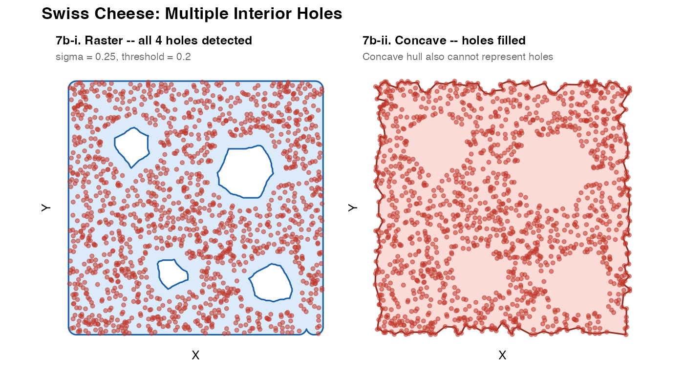

7c – Archipelago: disconnected islands

mk_isl <- function(n, cx, cy, rx, ry, ns = 0.15) {
  th <- runif(n, 0, 2 * pi)
  r  <- sqrt(runif(n))
  data.frame(x = cx + r * rx * cos(th) + rnorm(n, 0, ns),
             y = cy + r * ry * sin(th) + rnorm(n, 0, ns))
}
coords_arch <- rbind(mk_isl(300,  0,  0, 3,   2),
                     mk_isl(300,  9,  4, 2,   3),
                     mk_isl(300,  5, -7, 2.5, 1.5))

m7c_r <- fit_spatial_mask(coords_arch, method = "raster",
  raster_resolution = 256L, raster_sigma = 0.4, raster_threshold = 0.18,
  verbose = FALSE)
m7c_c <- fit_spatial_mask(coords_arch, method = "convex", verbose = FALSE)

n_geom <- length(sf::st_cast(m7c_r, "POLYGON"))

plot_mask(m7c_r, coords_arch,
          title    = sprintf("7c-i. Raster -- %d separate polygons", n_geom),
          subtitle = "Each island detected independently") +
plot_mask(m7c_c, coords_arch,
          title    = "7c-ii. Convex -- islands bridged",
          subtitle  = "Convex hull merges all islands into one",
          fill = "#e74c3c", border = "#922b21") +
plot_annotation(
  title = "Archipelago: Disconnected Islands",
  theme = theme(plot.title = element_text(face = "bold", size = 13)))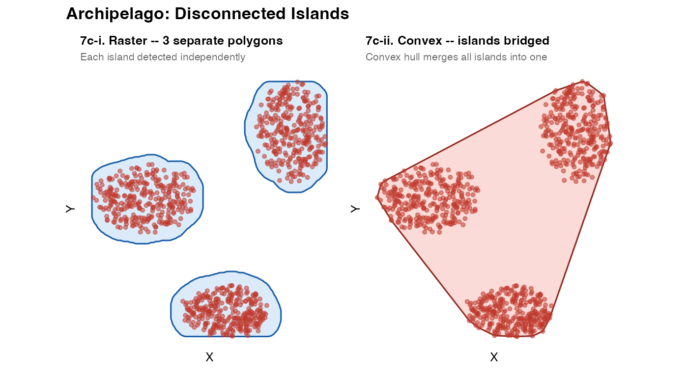

Disconnected islands emerge automatically from the GEOS union step: if two groups of “on” cells are not touching, they become separate polygons within the same sfc object. The number of distinct polygons is accessible via length(sf::st_cast(mask, "POLYGON")).

7d – Sigma sensitivity sweep

This is the most important tuning exercise. Run it on your own data before finalising raster_sigma.

sig_vals <- c(0.1, 0.2, 0.4, 0.7)
sig_cols <- c("#e74c3c", "#e67e22", "#27ae60", "#2980b9")

sig_pls <- mapply(function(sv, col) {
  m  <- fit_spatial_mask(coords_swiss, method = "raster",
    raster_resolution = 256L, raster_sigma = sv,
    raster_threshold  = 0.2,  verbose = FALSE)
  nh <- max(0L, length(sf::st_cast(m, "POLYGON")) - 1L)
  plot_mask(m, coords_swiss,
            title    = paste0("sigma = ", sv, " coord units"),
            subtitle = paste0(nh, " hole(s) detected"),
            fill = col, border = col, pt_size = 0.5)
}, sig_vals, sig_cols, SIMPLIFY = FALSE)

wrap_plots(sig_pls, nrow = 1) +
  plot_annotation(
    title    = "7d: raster_sigma Sensitivity -- Swiss Cheese",
    subtitle = "Small sigma -> holes preserved | Large sigma -> holes filled",
    theme    = theme(plot.title    = element_text(face = "bold", size = 13),
                     plot.subtitle = element_text(size = 9, color = "grey40")))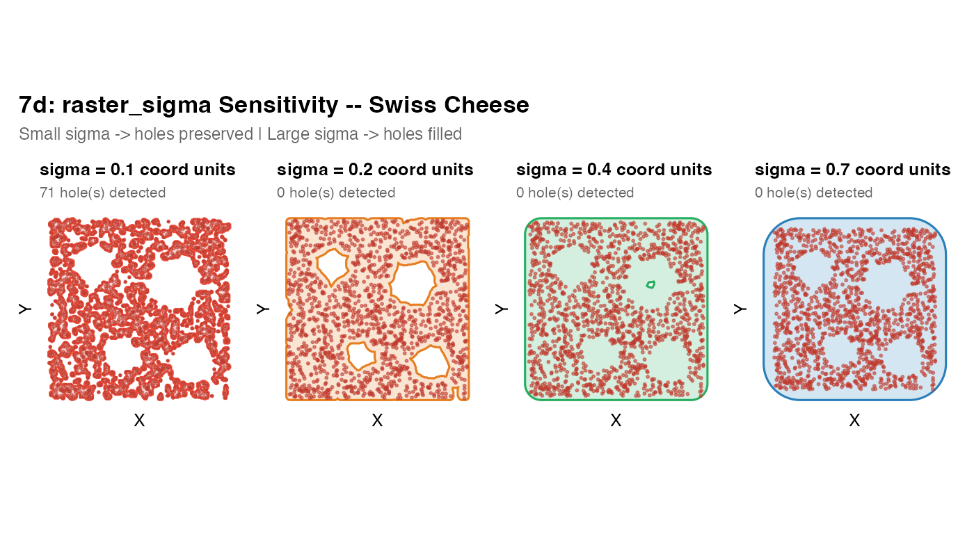

Tuning strategy:

Start with raster_sigma = NULL (auto = 3% of domain width)
Inspect the result; note whether real voids are detected
Decrease sigma if holes are being filled that you expect to be present
Increase sigma if the mask is too jagged or breaks into spurious fragments where there is actually continuous tissue
Adjust raster_threshold to expand or contract the mask after sigma is set

7e – Nested crescent voids

mk_cres <- function(cx, cy, ro, ri, dx, dy, n = 100) {
  moc <- .circle_mat(cx,    cy,    ro, n)
  mic <- .circle_mat(cx+dx, cy+dy, ri, n)
  oc  <- sf::st_polygon(list(moc))
  ic  <- sf::st_polygon(list(mic))
  sf::st_sfc(sf::st_difference(sf::st_sfc(oc), sf::st_sfc(ic)))
}

th_od  <- seq(0, 2 * pi, length.out = 200)
mat_od <- cbind(10 * cos(th_od), 10 * sin(th_od))
mat_od <- rbind(mat_od, mat_od[1L, ])
outer_d       <- sf::st_sfc(sf::st_polygon(list(mat_od)))
cres1         <- mk_cres(-2, 2,  2.5, 2,   0.9, -0.2)
cres2         <- mk_cres( 3, -3, 2.2, 1.8, -0.7,  0.4)
nest_region   <- sf::st_difference(outer_d, sf::st_union(c(cres1, cres2)))
coords_nested <- sample_in_polygon(nest_region, n = 2500)

m7e_fine   <- fit_spatial_mask(coords_nested, method = "raster",
  raster_resolution = 256L, raster_sigma = 0.4,  raster_threshold = 0.18,
  verbose = FALSE)
m7e_coarse <- fit_spatial_mask(coords_nested, method = "raster",
  raster_resolution = 256L, raster_sigma = 1.0, raster_threshold = 0.18,
  verbose = FALSE)

plot_mask(m7e_fine,   coords_nested,
          title    = "7e-i. Fine sigma = 0.4",
          subtitle = "Crescent voids preserved") +
plot_mask(m7e_coarse, coords_nested,
          title    = "7e-ii. Coarse sigma = 1.0",
          subtitle = "Narrow voids filled in",
          fill = "#8e44ad", border = "#6c3483") +
plot_annotation(
  title    = "Nested Crescent Voids: sigma controls void resolution",
  subtitle = "The minimum detectable void width is approximately 2 x raster_sigma",
  theme    = theme(plot.title    = element_text(face = "bold", size = 13),
                   plot.subtitle = element_text(size = 9, color = "grey40")))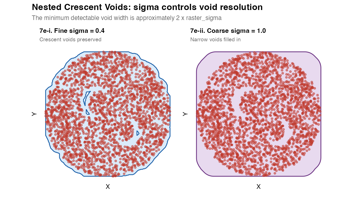

Key principle: The minimum resolvable void has a width of approximately 2 x raster_sigma. Voids narrower than this will be filled in by the Gaussian blur. If you need to resolve fine voids (e.g. individual capillary lumens), you must use a small sigma – but this may also make the mask jagged elsewhere.

7f – Scale test: 100,000 cells

The raster method is O(N^2) in the grid size but O(n) in the number of input points (binning is a single tabulate() call). This makes it practical for large datasets.

th100    <- seq(0, 2 * pi, length.out = 400)
r100     <- 12 + sin(5 * th100) + 0.4 * cos(11 * th100)
mat100   <- cbind(r100 * cos(th100), r100 * sin(th100))
mat100   <- rbind(mat100, mat100[1L, ])
outer100 <- sf::st_sfc(sf::st_polygon(list(mat100)))

make_ellipse_poly <- function(cx, cy, a, b, angle_deg, n = 80) {
  th  <- seq(0, 2 * pi, length.out = n)
  ang <- angle_deg * pi / 180
  xe  <- a * cos(th); ye <- b * sin(th)
  mat <- cbind(cx + xe * cos(ang) - ye * sin(ang),
               cy + xe * sin(ang) + ye * cos(ang))
  mat <- rbind(mat, mat[1L, ])
  sf::st_polygon(list(mat))
}

holes100 <- sf::st_sfc(list(
  make_ellipse_poly( 3,  5,  3,   1.5,  10),
  make_ellipse_poly(-5,  2,  2.5, 2,   -30),
  make_ellipse_poly( 1, -6,  2,   3,    50)
))
reg100      <- sf::st_difference(outer100, sf::st_union(holes100))
coords_100k <- sample_in_polygon(reg100, n = 100000)

t_raster <- system.time(
  m_100k <- fit_spatial_mask(coords_100k, method = "raster",
    raster_resolution = 256L, raster_sigma = 0.6,
    raster_threshold  = 0.18, verbose = TRUE)
)

## --------------------------------------------------
##   TissueMask: spatial mask fitted
##   Method         : raster 
##   Points         : 100000 
##   Sub-geometries : 1 
##   Bounding box   : x [ -12.93 , 12.629 ]  y [ -11.827 , 13.227 ]
##   Area           : 523.5807 
##   Buffer applied : 0 
## --------------------------------------------------

sub <- coords_100k[sample(nrow(coords_100k), 5000), ]
plot_mask(m_100k, sub,
          title    = sprintf("7f. 100k cells -- raster (%.1f s)", t_raster["elapsed"]),
          subtitle = "3 elliptic holes detected | 5,000 of 100,000 points shown",
          pt_size  = 0.3, pt_alpha = 0.2)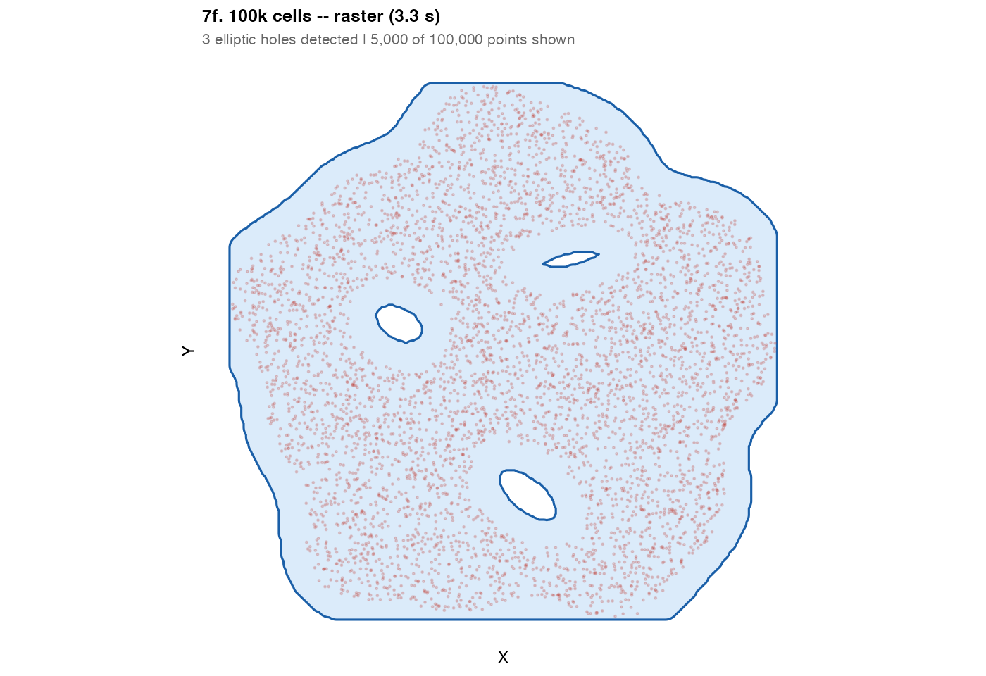

Section 8 – Validation: point containment

A properly fitted mask must contain all its input points. This table checks every mask produced in this vignette. Any FAIL indicates that the mask needs a larger buffer_dist or a lower raster_threshold.

cases <- list(
  list(label = "Circle/convex",      mask = m1a,       coords = coords_circle),
  list(label = "Circle/concave",     mask = m1b,       coords = coords_circle),
  list(label = "Circle/kde",         mask = m1c,       coords = coords_circle),
  list(label = "Elongated/convex",   mask = m2a,       coords = coords_elong),
  list(label = "Elongated/concave",  mask = m2b,       coords = coords_elong),
  list(label = "Elongated/kde",      mask = m2c,       coords = coords_elong),
  list(label = "L-shape/convex",     mask = m3a,       coords = coords_L),
  list(label = "L-shape/conc1.5",    mask = m3b,       coords = coords_L),
  list(label = "L-shape/conc3",      mask = m3c,       coords = coords_L),
  list(label = "Multi/convex",       mask = m4a,       coords = coords_multi),
  list(label = "Multi/concave",      mask = m4b,       coords = coords_multi),
  list(label = "Multi/kde-lo",       mask = m4c,       coords = coords_multi),
  list(label = "Multi/kde-hi",       mask = m4d,       coords = coords_multi),
  list(label = "Ring/raw",           mask = m6a,       coords = coords_ring),
  list(label = "Ring/buffer",        mask = m6b,       coords = coords_ring),
  list(label = "Ring/smooth",        mask = m6c,       coords = coords_ring),
  list(label = "Donut/raster",       mask = m7a_r,     coords = coords_donut),
  list(label = "Swiss/raster",       mask = m7b_r,     coords = coords_swiss),
  list(label = "Archipelago/raster", mask = m7c_r,     coords = coords_arch),
  list(label = "Nested/fine",        mask = m7e_fine,  coords = coords_nested),
  list(label = "Nested/coarse",      mask = m7e_coarse,coords = coords_nested),
  list(label = "100k/raster",        mask = m_100k,    coords = coords_100k)
)

results <- do.call(rbind, lapply(cases, function(vc) {
  pts <- sf::st_geometry(sf::st_as_sf(vc$coords, coords = c("x","y")))
  ok  <- sf::st_covered_by(pts, sf::st_union(vc$mask), sparse = FALSE)[, 1L]
  n   <- nrow(vc$coords)
  data.frame(
    Case     = vc$label,
    N        = n,
    Enclosed = sum(ok),
    Pct      = round(100 * sum(ok) / n, 2),
    Result   = ifelse(sum(ok) == n, "PASS", "FAIL"),
    stringsAsFactors = FALSE
  )
}))

knitr::kable(results, align = c("l","r","r","r","c"))

Case	N	Enclosed	Pct	Result
Circle/convex	400	400	100	PASS
Circle/concave	400	400	100	PASS
Circle/kde	400	400	100	PASS
Elongated/convex	400	400	100	PASS
Elongated/concave	400	400	100	PASS
Elongated/kde	400	400	100	PASS
L-shape/convex	400	400	100	PASS
L-shape/conc1.5	400	400	100	PASS
L-shape/conc3	400	400	100	PASS
Multi/convex	450	450	100	PASS
Multi/concave	450	450	100	PASS
Multi/kde-lo	450	450	100	PASS
Multi/kde-hi	450	450	100	PASS
Ring/raw	250	250	100	PASS
Ring/buffer	250	250	100	PASS
Ring/smooth	250	250	100	PASS
Donut/raster	800	800	100	PASS
Swiss/raster	1500	1500	100	PASS
Archipelago/raster	900	900	100	PASS
Nested/fine	2500	2500	100	PASS
Nested/coarse	2500	2500	100	PASS
100k/raster	100000	100000	100	PASS

Quick-start decision guide

Your data
  |
  +-- Simple convex blob? -----------------------> method = "convex"
  |
  +-- Non-convex (C-shape, arc, L-shape)?
  |   +-- No holes needed? -------------------> method = "concave"
  |                                             concavity: start at 2, lower to tighten
  |
  +-- Holes or islands expected?
  |   +-- n < 50,000? -----------------------> method = "raster"
  |   +-- n > 50,000? -----------------------> method = "raster" (still fine)
  |
  +-- Dense, smooth, no need for holes?
      +-- KDE is an alternative -------------> method = "kde"
                                               kde_threshold: start at 0.05

For method = "raster":
  raster_sigma   = NULL  (auto) for a first pass
  raster_sigma smaller: preserve fine voids
  raster_sigma larger:  fill gaps and smooth edges
  raster_threshold = 0.15 is a reliable default

Session information

sessionInfo()

## R version 4.5.2 (2025-10-31)
## Platform: aarch64-apple-darwin20
## Running under: macOS Sonoma 14.6.1
## 
## Matrix products: default
## BLAS:   /System/Library/Frameworks/Accelerate.framework/Versions/A/Frameworks/vecLib.framework/Versions/A/libBLAS.dylib 
## LAPACK: /Library/Frameworks/R.framework/Versions/4.5-arm64/Resources/lib/libRlapack.dylib;  LAPACK version 3.12.1
## 
## locale:
## [1] en_US/en_US/en_US/C/en_US/en_US
## 
## time zone: America/New_York
## tzcode source: internal
## 
## attached base packages:
## [1] stats     graphics  grDevices utils     datasets  methods   base     
## 
## other attached packages:
## [1] patchwork_1.3.2  ggplot2_4.0.1    sf_1.0-21        TissueMask_0.1.0
## 
## loaded via a namespace (and not attached):
##  [1] sass_0.4.10        generics_0.1.4     class_7.3-23       KernSmooth_2.23-26
##  [5] digest_0.6.39      magrittr_2.0.4     evaluate_1.0.5     grid_4.5.2        
##  [9] RColorBrewer_1.1-3 fastmap_1.2.0      jsonlite_2.0.0     e1071_1.7-16      
## [13] DBI_1.2.3          scales_1.4.0       isoband_0.3.0      textshaping_1.0.1 
## [17] jquerylib_0.1.4    cli_3.6.5          rlang_1.1.7        units_0.8-7       
## [21] withr_3.0.2        cachem_1.1.0       yaml_2.3.12        otel_0.2.0        
## [25] concaveman_1.2.0   tools_4.5.2        parallel_4.5.2     dplyr_1.1.4       
## [29] curl_7.0.0         vctrs_0.7.1        R6_2.6.1           proxy_0.4-27      
## [33] lifecycle_1.0.5    classInt_0.4-11    V8_8.0.1           fs_1.6.6          
## [37] htmlwidgets_1.6.4  MASS_7.3-65        ragg_1.4.0         pkgconfig_2.0.3   
## [41] desc_1.4.3         pkgdown_2.1.3      bslib_0.10.0       pillar_1.11.1     
## [45] gtable_0.3.6       glue_1.8.0         Rcpp_1.1.1         systemfonts_1.2.3 
## [49] xfun_0.56          tibble_3.3.1       tidyselect_1.2.1   knitr_1.51        
## [53] dichromat_2.0-0.1  farver_2.1.2       htmltools_0.5.9    rmarkdown_2.30    
## [57] compiler_4.5.2     S7_0.2.1

Methods, parameters, and tuning across all use cases

Raredon Laboratory, Yale School of Medicine

2026-04-04

Overview

Setup

Shared plotting helper

Function reference: `fit_spatial_mask()`

Return value

Section 1 — Circular cloud: sanity check

Section 2 – Elongated cloud: anisotropy

Section 3 – L-shaped cloud: the non-convex diagnostic

The `concavity` parameter

Section 4 – Multi-cluster blobs: connected vs. isolated masks

Choosing `kde_threshold`

Section 5 – Concavity sweep on a crescent

Section 6 – Buffer and smoothing

Section 7 – Topologically complex cases: holes and islands

How the raster method works

Key tuning parameters

7a – Donut: single interior void

7b – Swiss cheese: multiple holes

7c – Archipelago: disconnected islands

7d – Sigma sensitivity sweep

7e – Nested crescent voids

7f – Scale test: 100,000 cells

Section 8 – Validation: point containment

Quick-start decision guide

Session information

Complete Reference: fit_spatial_mask()

Methods, parameters, and tuning across all use cases

Raredon Laboratory, Yale School of Medicine

2026-04-04

Overview

Setup

Shared plotting helper

Function reference: fit_spatial_mask()

Return value

Section 1 — Circular cloud: sanity check

Section 2 – Elongated cloud: anisotropy

Section 3 – L-shaped cloud: the non-convex diagnostic

The concavity parameter

Section 4 – Multi-cluster blobs: connected vs. isolated masks

Choosing kde_threshold

Section 5 – Concavity sweep on a crescent

Section 6 – Buffer and smoothing

Section 7 – Topologically complex cases: holes and islands

How the raster method works

Key tuning parameters

7a – Donut: single interior void

7b – Swiss cheese: multiple holes

7c – Archipelago: disconnected islands

7d – Sigma sensitivity sweep

7e – Nested crescent voids

7f – Scale test: 100,000 cells

Section 8 – Validation: point containment

Quick-start decision guide

Session information

Function reference: `fit_spatial_mask()`

The `concavity` parameter

Choosing `kde_threshold`