Beta-Catenin Knockout Analysis with PathwayEmbed
beta_catenin_ko_updated.RmdOverview
This vignette demonstrates the application of PathwayEmbed in a beta-catenin perturbed system where the Ctnnb1 upstream enhancer is depleted in intestinal epithelia. Because the KO genotype is known by design, this dataset provides a clean biological ground truth for a direct AUROC benchmark against PROGENy and AddModuleScore.
Reference: Hua et al., eLife 13: RP98238 (2024). https://doi.org/10.7554/eLife.98238
Load Packages
library(PathwayEmbed)
library(Seurat)
library(ggplot2)
library(patchwork)
library(pheatmap)
library(progeny)
library(pROC)
Helper: Annotation Label Builder
make_label <- function(stats, group1, group2) {
  d    <- round(stats$cohens_d[1], 3)
  p    <- formatC(stats$p_value[1], format = "e", digits = 2)
  on1  <- stats$percentage_on[stats$group  == group1]
  off1 <- stats$percentage_off[stats$group == group1]
  on2  <- stats$percentage_on[stats$group  == group2]
  off2 <- stats$percentage_off[stats$group == group2]
  paste0(
    group1, ": ON=", on1,  "%, OFF=", off1, "%\n",
    group2, ": ON=", on2,  "%, OFF=", off2, "%\n",
    "Cohen's d = ", d, "\n",
    "p = ", p
  )
}
Download Data
url_ko <- "https://ftp.ncbi.nlm.nih.gov/geo/series/GSE233nnn/GSE233978/suppl/GSE233978_KO_filtered_feature_bc_matrix.h5"
url_wt <- "https://ftp.ncbi.nlm.nih.gov/geo/series/GSE233nnn/GSE233978/suppl/GSE233978_WT_filtered_feature_bc_matrix.h5"

download.file(url_ko, destfile = "GSE233978_KO_filtered_feature_bc_matrix.h5", mode = "wb")
download.file(url_wt, destfile = "GSE233978_WT_filtered_feature_bc_matrix.h5", mode = "wb")
Data Preparation and Preprocessing
ko_data <- Read10X_h5("GSE233978_KO_filtered_feature_bc_matrix.h5")
wt_data <- Read10X_h5("GSE233978_WT_filtered_feature_bc_matrix.h5")

ko <- CreateSeuratObject(counts = ko_data, project = "KO",
                          min.cells = 3, min.features = 200)
wt <- CreateSeuratObject(counts = wt_data, project = "WT",
                          min.cells = 3, min.features = 200)
ko$sample <- "KO"
wt$sample <- "WT"

merged          <- merge(ko, wt)
merged[["RNA"]] <- JoinLayers(merged[["RNA"]])

merged <- NormalizeData(merged, normalization.method = "LogNormalize",
                         scale.factor = 10000)
merged <- FindVariableFeatures(merged, selection.method = "vst",
                                nfeatures = 2000)
merged <- ScaleData(merged, features = VariableFeatures(merged))
Wnt Pathway Scoring
Wnt_12h   <- LoadPathway("WNT3A_12H_ACTIVATION",  "mouse")
Wnt_24h   <- LoadPathway("WNT3A_24H_ACTIVATION",  "mouse")
Wnt_48h   <- LoadPathway("WNT3A_48H_ACTIVATION",  "mouse")
Wnt_slope <- LoadPathway("WNT3A_SLOPE_ACTIVATION", "mouse")

matrix_12h   <- DataPreProcess(merged, Wnt_12h,   Seurat.object = TRUE)
matrix_24h   <- DataPreProcess(merged, Wnt_24h,   Seurat.object = TRUE)
matrix_48h   <- DataPreProcess(merged, Wnt_48h,   Seurat.object = TRUE)
matrix_slope <- DataPreProcess(merged, Wnt_slope, Seurat.object = TRUE)

pathwaystat_12h   <- PathwayMaxMin(matrix_12h,   Wnt_12h)
pathwaystat_24h   <- PathwayMaxMin(matrix_24h,   Wnt_24h)
pathwaystat_48h   <- PathwayMaxMin(matrix_48h,   Wnt_48h)
pathwaystat_slope <- PathwayMaxMin(matrix_slope, Wnt_slope)

score_12h   <- ComputeCellData(matrix_12h,   pathwaystat_12h)
score_24h   <- ComputeCellData(matrix_24h,   pathwaystat_24h)
score_48h   <- ComputeCellData(matrix_48h,   pathwaystat_48h)
score_slope <- ComputeCellData(matrix_slope, pathwaystat_slope)
Visualization
plot_data_12h <- PreparePlotData(merged, score_12h, "sample", Seurat.object = TRUE)
plot_data_24h <- PreparePlotData(merged, score_24h, "sample", Seurat.object = TRUE)
plot_data_48h <- PreparePlotData(merged, score_48h, "sample", Seurat.object = TRUE)
plot_data_slope <- PreparePlotData(merged, score_slope, "sample", Seurat.object = TRUE)
pct_12h <- CalculatePercentage(plot_data_12h, "sample")
pct_24h <- CalculatePercentage(plot_data_24h, "sample")
pct_48h <- CalculatePercentage(plot_data_48h, "sample")
pct_slope <- CalculatePercentage(plot_data_slope, "sample")
pct_12h; pct_24h; pct_48h; pct_slope
#> # A tibble: 2 × 5
#> group percentage_on percentage_off cohens_d p_value
#> <chr> <dbl> <dbl> <dbl> <dbl>
#> 1 KO 50.5 49.5 -0.0728 2.50e-12
#> 2 WT 53.6 46.4 -0.0728 2.50e-12
#> # A tibble: 2 × 5
#> group percentage_on percentage_off cohens_d p_value
#> <chr> <dbl> <dbl> <dbl> <dbl>
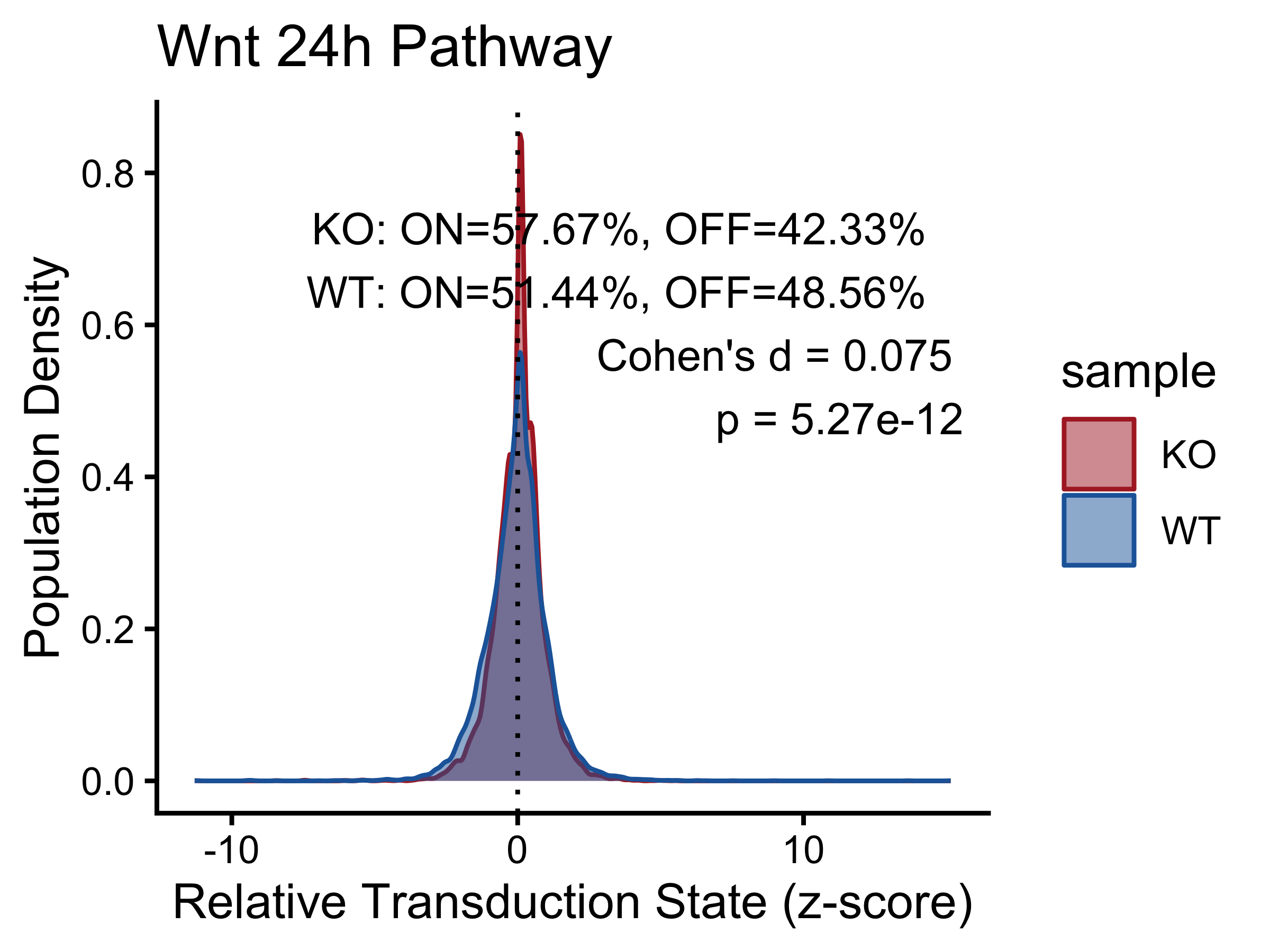
#> 1 KO 57.7 42.3 0.0748 5.27e-12
#> 2 WT 51.4 48.6 0.0748 5.27e-12
#> # A tibble: 2 × 5
#> group percentage_on percentage_off cohens_d p_value
#> <chr> <dbl> <dbl> <dbl> <dbl>
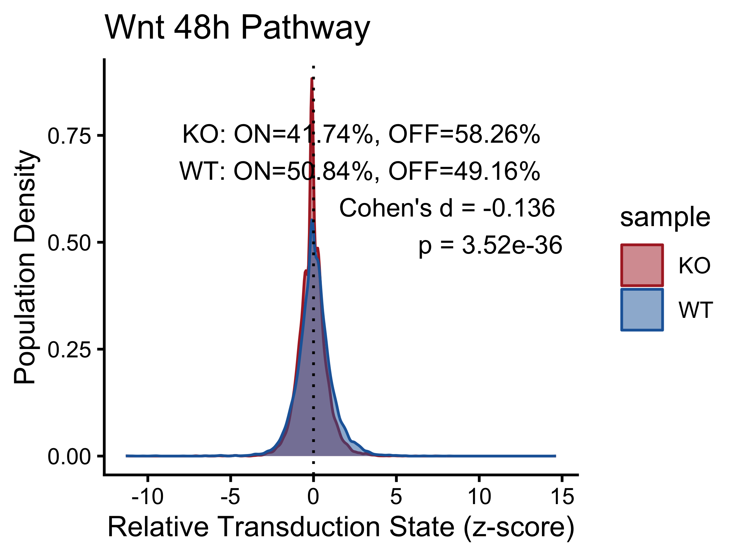
#> 1 KO 41.7 58.3 -0.136 3.52e-36
#> 2 WT 50.8 49.2 -0.136 3.52e-36
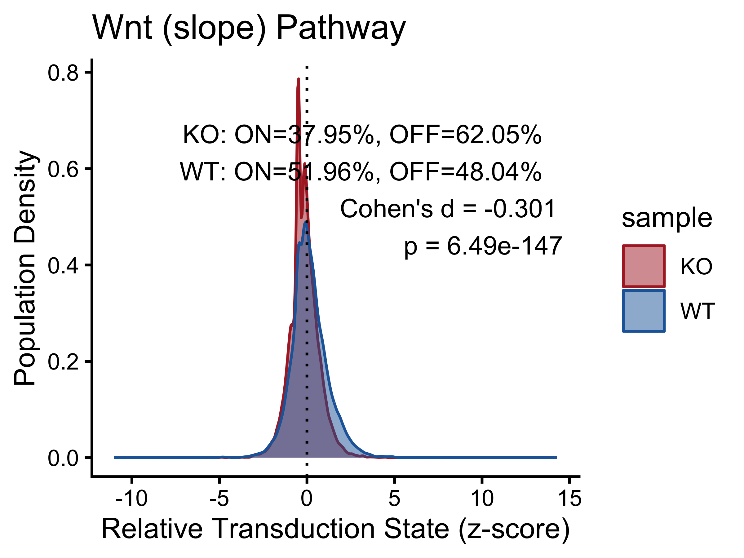
#> # A tibble: 2 × 5
#> group percentage_on percentage_off cohens_d p_value
#> <chr> <dbl> <dbl> <dbl> <dbl>
#> 1 KO 38.0 62.0 -0.301 6.49e-147
#> 2 WT 52.0 48.0 -0.301 6.49e-147
p_12h <- PlotPathway(plot_data_12h, "Wnt 12h", "sample", c("#ae282c", "#2066a8")) +
annotate("text", x = Inf, y = Inf, hjust = 1.1, vjust = 1.5,
label = make_label(pct_12h, "KO", "WT"), size = 3.5, color = "black")
p_24h <- PlotPathway(plot_data_24h, "Wnt 24h", "sample", c("#ae282c", "#2066a8")) +
annotate("text", x = Inf, y = Inf, hjust = 1.1, vjust = 1.5,
label = make_label(pct_24h, "KO", "WT"), size = 3.5, color = "black")
p_48h <- PlotPathway(plot_data_48h, "Wnt 48h", "sample", c("#ae282c", "#2066a8")) +
annotate("text", x = Inf, y = Inf, hjust = 1.1, vjust = 1.5,
label = make_label(pct_48h, "KO", "WT"), size = 3.5, color = "black")
p_slope <- PlotPathway(plot_data_slope, "Wnt (slope)", "sample", c("#ae282c", "#2066a8")) +
annotate("text", x = Inf, y = Inf, hjust = 1.1, vjust = 1.5,
label = make_label(pct_slope, "KO", "WT"), size = 3.5, color = "black")
p_12h; p_24h; p_48h; p_slope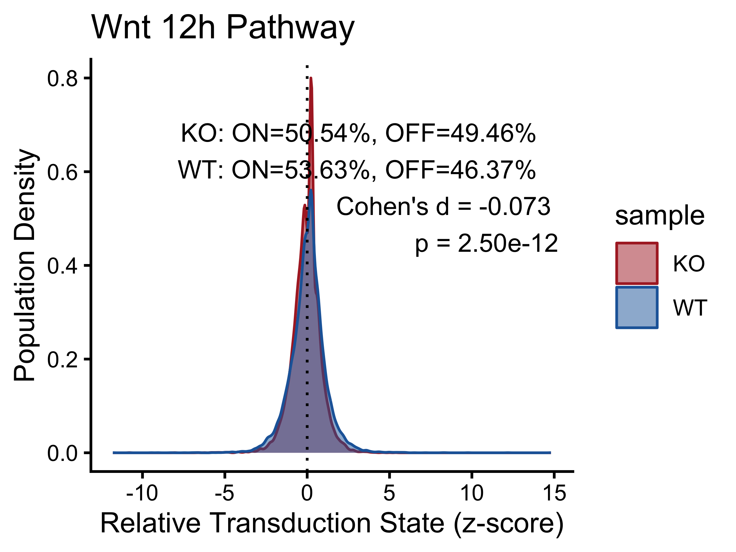
Technical Confounders
merged[["percent.mt"]] <- PercentageFeatureSet(merged, pattern = "^mt-")
seurat_meta <- merged@meta.data

make_scatter <- function(df, x_col, x_label) {
  r <- cor(df$embed_score, df[[x_col]], method = "spearman", use = "complete.obs")
  ggplot(df, aes(x = .data[[x_col]], y = embed_score)) +
    geom_point(alpha = 0.3, size = 0.8, color = "#534AB7") +
    geom_smooth(method = "lm", color = "#E24B4A", linewidth = 0.8, se = TRUE) +
    labs(title = sprintf("%s (rho = %.3f)", x_label, r),
         x = x_label, y = "PathwayEmbed score") +
    theme_minimal()
}

confounder_df <- data.frame(
  cell         = names(score_slope),
  embed_score  = as.numeric(score_slope),
  nCount_RNA   = seurat_meta[names(score_slope), "nCount_RNA"],
  nFeature_RNA = seurat_meta[names(score_slope), "nFeature_RNA"],
  percent_mt   = seurat_meta[names(score_slope), "percent.mt"]
)

for (cov in c("nCount_RNA", "nFeature_RNA", "percent_mt")) {
  r <- cor(confounder_df$embed_score, confounder_df[[cov]],
           method = "spearman", use = "complete.obs")
  cat(sprintf("Spearman vs %-15s : %.3f\n", cov, r))
}
#> Spearman vs nCount_RNA      : 0.188
#> Spearman vs nFeature_RNA    : 0.262
#> Spearman vs percent_mt      : -0.119

(make_scatter(confounder_df, "nCount_RNA",   "nCount_RNA") +
 make_scatter(confounder_df, "nFeature_RNA", "nFeature_RNA") +
 make_scatter(confounder_df, "percent_mt",   "percent.mt"))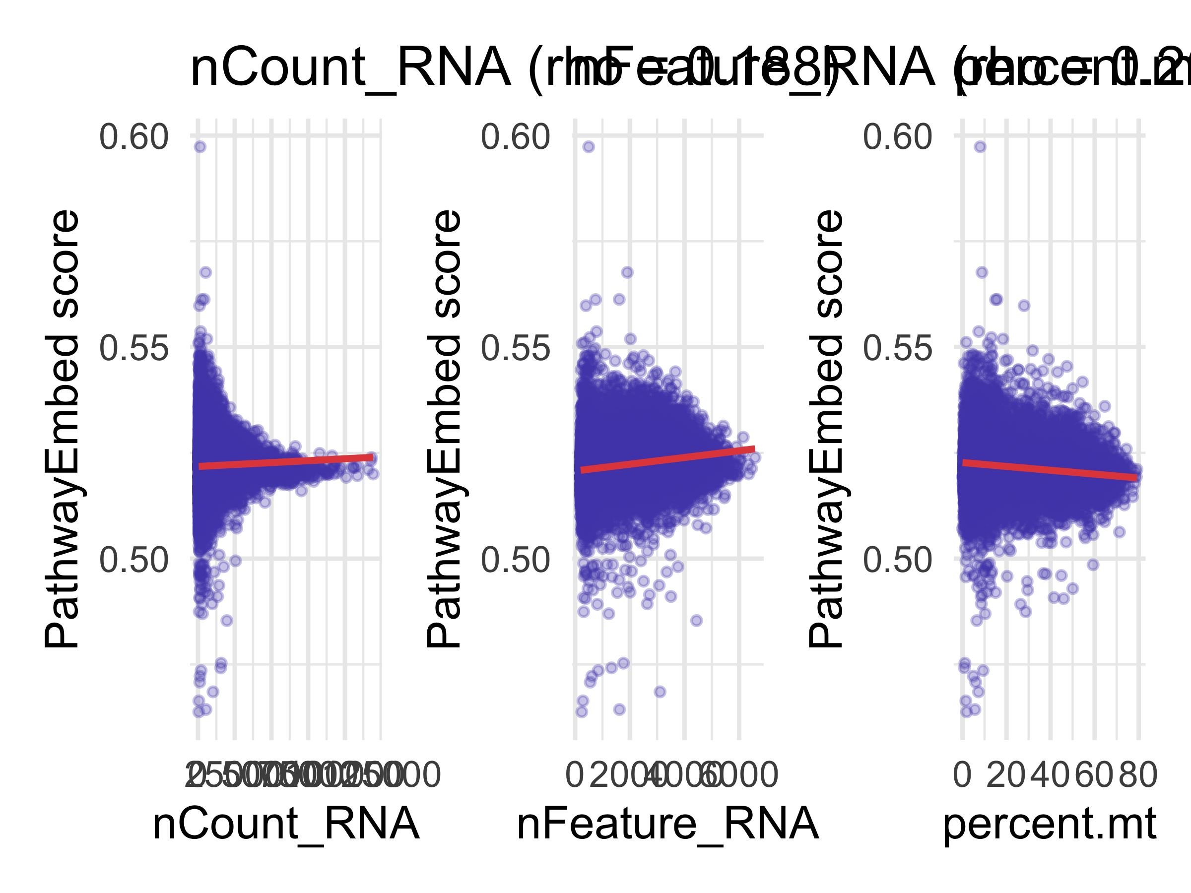
Benchmark Against PROGENy and AddModuleScore
normalized_mat       <- GetAssayData(merged, assay = "RNA", layer = "data")
normalized_mat_dense <- as.matrix(normalized_mat)

common_genes         <- intersect(rownames(normalized_mat_dense), Wnt_slope$Gene_Symbol)
gene_matrix          <- normalized_mat_dense[common_genes, ]
mean_expr            <- colMeans(gene_matrix, na.rm = TRUE)
zscore_mean_per_cell <- colMeans(t(scale(t(gene_matrix))), na.rm = TRUE)

progeny_scores <- progeny(
  normalized_mat_dense,
  scale    = TRUE,
  organism = "Mouse",
  top      = 100,
  perm     = 1
)
progeny_wnt <- setNames(as.numeric(progeny_scores[, "WNT"]),
                         rownames(progeny_scores))

wnt_features <- rownames(matrix_slope)
merged <- AddModuleScore(
  object   = merged,
  features = list(wnt_features),
  name     = "WNT_ModuleScore",
  ctrl     = 5,
  nbin     = 10
)
module_score <- setNames(
  merged@meta.data$WNT_ModuleScore1,
  rownames(merged@meta.data)
)

cells <- names(score_slope)
benchmark_df <- data.frame(
  PathwayEmbed   = as.numeric(score_slope),
  PROGENy        = as.numeric(progeny_wnt[cells]),
  AddModuleScore = as.numeric(module_score[cells]),
  mean_expr      = as.numeric(mean_expr[cells]),
  zscore_expr    = as.numeric(zscore_mean_per_cell[cells]),
  row.names      = cells
)

benchmark_cor <- cor(benchmark_df, method = "spearman",
                     use = "pairwise.complete.obs")
print(round(benchmark_cor, 3))
#>                PathwayEmbed PROGENy AddModuleScore mean_expr zscore_expr
#> PathwayEmbed          1.000   0.095          0.106     0.359       0.356
#> PROGENy               0.095   1.000         -0.180     0.367       0.362
#> AddModuleScore        0.106  -0.180          1.000     0.146       0.139
#> mean_expr             0.359   0.367          0.146     1.000       0.972
#> zscore_expr           0.356   0.362          0.139     0.972       1.000

p_cor <- pheatmap(
  benchmark_cor,
  color           = colorRampPalette(c("#185FA5", "white", "#993C1D"))(100),
  breaks          = seq(-1, 1, length.out = 101),
  display_numbers = TRUE, number_format = "%.2f",
  fontsize_number = 9,
  main            = "Method Benchmark — Spearman Correlation (Ctnnb1 KO dataset)"
)
p_cor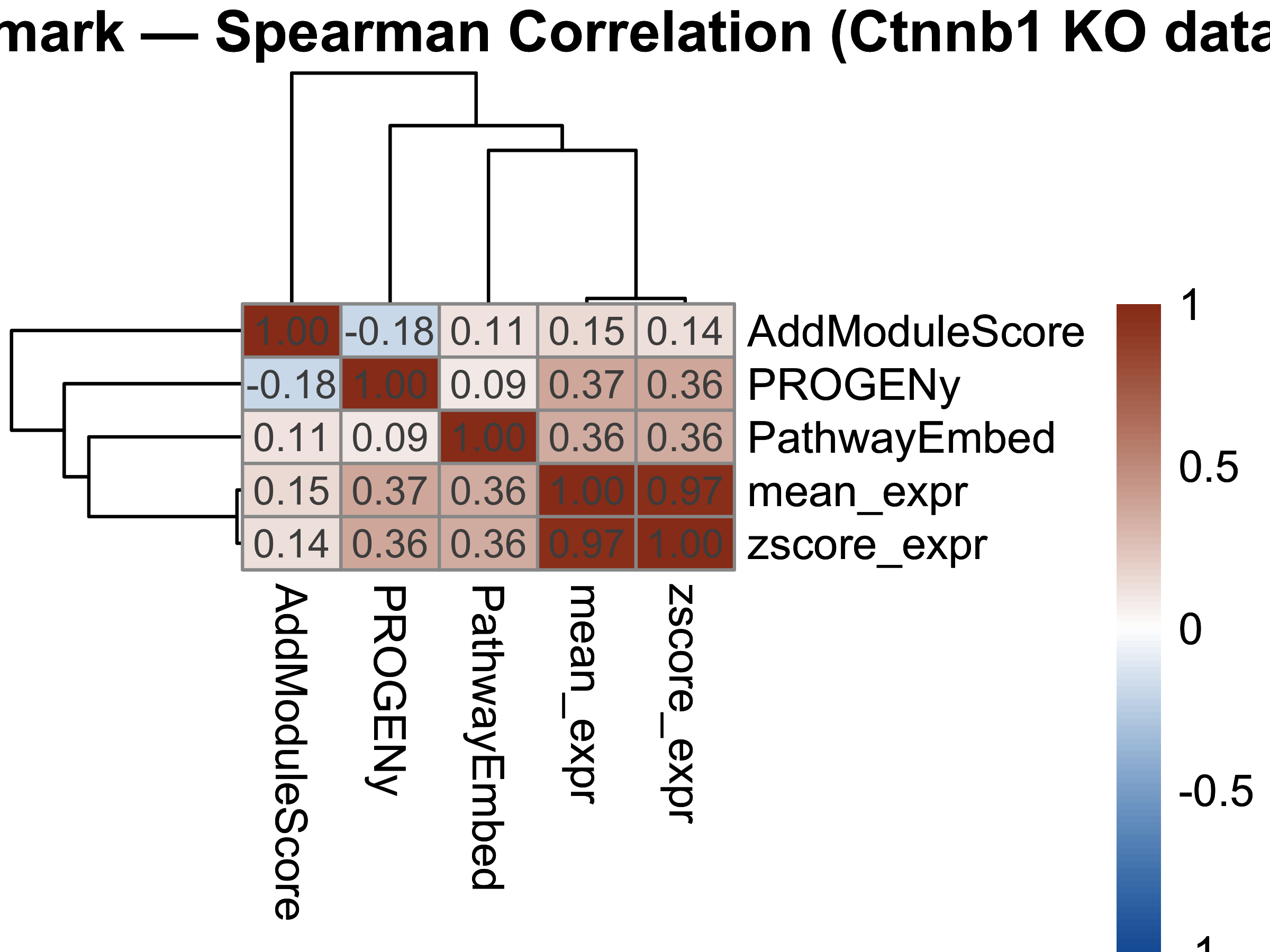
ko_label <- ifelse(merged@meta.data[cells, "sample"] == "KO", 1L, 0L)
compute_auroc <- function(scores, labels) {
r <- roc(labels, scores, quiet = TRUE)
auc_val <- as.numeric(auc(r))
if (auc_val < 0.5) auc_val <- 1 - auc_val
auc_val
}
auroc_results <- data.frame(
Method = colnames(benchmark_df),
AUROC = sapply(benchmark_df, compute_auroc, labels = ko_label)
)
auroc_results <- auroc_results[order(-auroc_results$AUROC), ]
print(auroc_results)
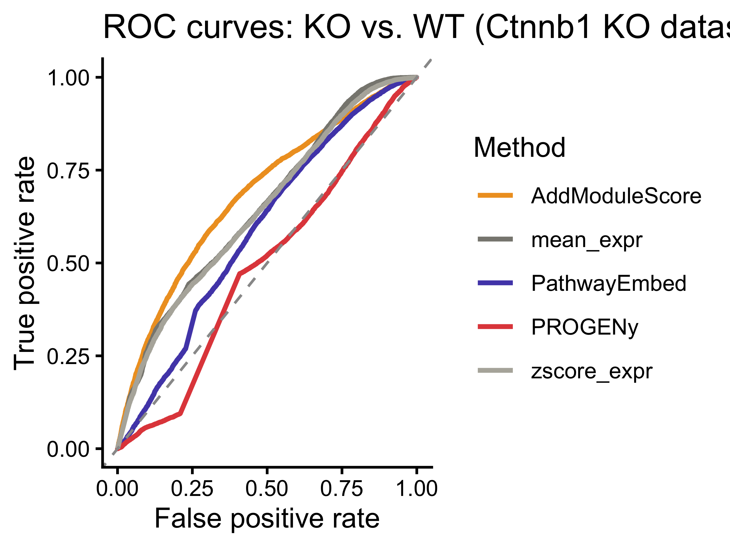
#> Method AUROC
#> AddModuleScore AddModuleScore 0.6827026
#> mean_expr mean_expr 0.6482098
#> zscore_expr zscore_expr 0.6425566
#> PathwayEmbed PathwayEmbed 0.5897700
#> PROGENy PROGENy 0.5106677
compute_cohens_d_method <- function(scores_vec, seurat_obj, group_col) {
pd <- PreparePlotData(seurat_obj, scores_vec, group_col, Seurat.object = TRUE)
pct <- CalculatePercentage(pd, group_var = group_col)
abs(pct$cohens_d[1])
}
cohens_d_results <- data.frame(
Method = colnames(benchmark_df),
Cohens_d = sapply(
colnames(benchmark_df),
function(m) {
sv <- setNames(benchmark_df[[m]], rownames(benchmark_df))
compute_cohens_d_method(sv, merged, "sample")
}
)
)
cohens_d_results <- cohens_d_results[order(-cohens_d_results$Cohens_d), ]
print(cohens_d_results)
#> Method Cohens_d
#> AddModuleScore AddModuleScore 0.64575350
#> mean_expr mean_expr 0.54020251
#> zscore_expr zscore_expr 0.51565732
#> PathwayEmbed PathwayEmbed 0.30056596
#> PROGENy PROGENy 0.03129493
method_colors <- c(
"PathwayEmbed" = "#534AB7",
"PROGENy" = "#E24B4A",
"AddModuleScore" = "#EF9F27",
"mean_expr" = "#888780",
"zscore_expr" = "#B4B2A9"
)
p_cd <- ggplot(cohens_d_results,
aes(x = reorder(Method, Cohens_d), y = Cohens_d, fill = Method)) +
geom_bar(stat = "identity", width = 0.6) +
coord_flip() +
scale_fill_manual(values = method_colors) +
labs(title = "Effect size (Cohen's d): KO vs. WT",
x = NULL, y = "Cohen's d (absolute)") +
theme_classic() +
theme(legend.position = "none")
p_cd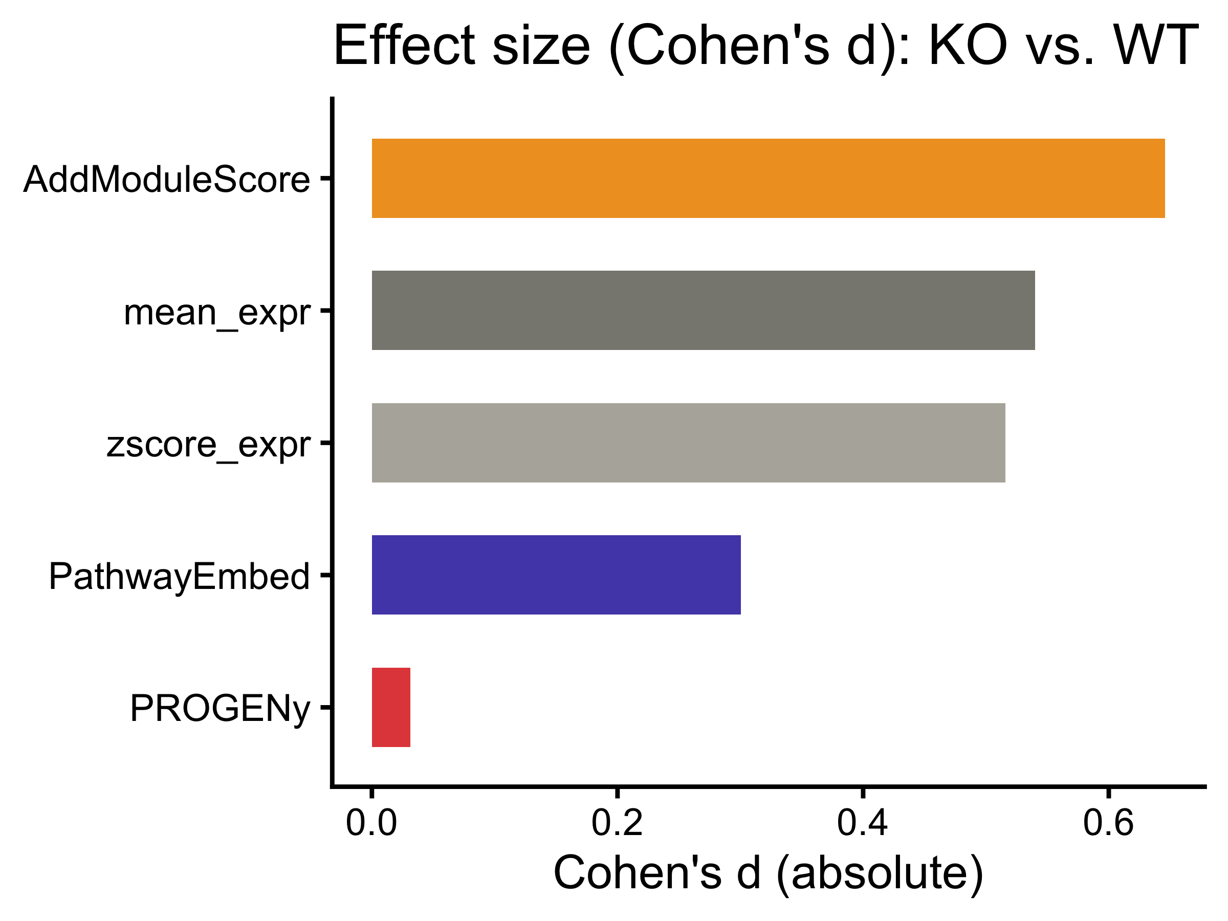
p_auroc <- ggplot(auroc_results,
       aes(x = reorder(Method, AUROC), y = AUROC, fill = Method)) +
  geom_bar(stat = "identity", width = 0.6) +
  geom_hline(yintercept = 0.5, linetype = "dashed", color = "black") +
  coord_flip() +
  scale_fill_manual(values = method_colors) +
  labs(title = "AUROC: KO vs. WT separation (Ctnnb1 KO dataset)",
       x = NULL, y = "AUROC") +
  ylim(0, 1) +
  theme_classic() +
  theme(legend.position = "none")
p_auroc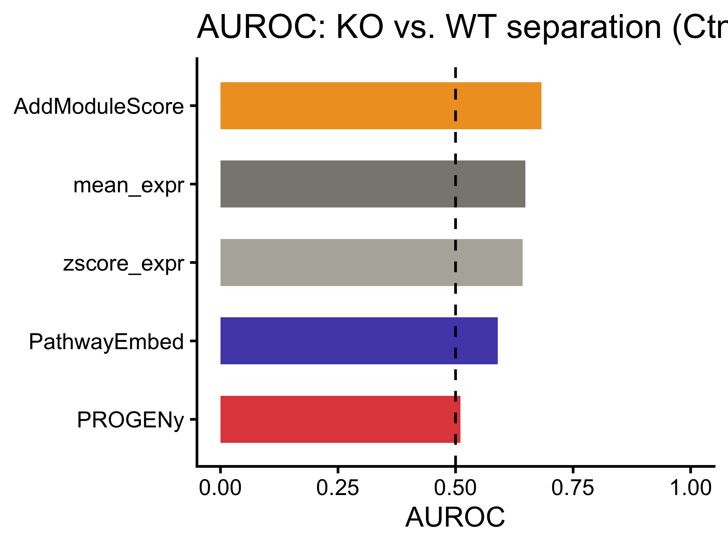
roc_list <- lapply(colnames(benchmark_df), function(m) {
  roc(ko_label, benchmark_df[[m]], quiet = TRUE)
})
names(roc_list) <- colnames(benchmark_df)

roc_df <- do.call(rbind, lapply(names(roc_list), function(m) {
  r <- roc_list[[m]]
  data.frame(Method = m, FPR = 1 - r$specificities, TPR = r$sensitivities)
}))

p_roc <- ggplot(roc_df, aes(x = FPR, y = TPR, color = Method)) +
  geom_line(linewidth = 0.9) +
  geom_abline(intercept = 0, slope = 1, linetype = "dashed", color = "grey60") +
  scale_color_manual(values = method_colors) +
  labs(title = "ROC curves: KO vs. WT (Ctnnb1 KO dataset)",
       x = "False positive rate", y = "True positive rate") +
  theme_classic()
p_roc