This tutorial runs a full spatial analysis on a public 10x Visium section of the mouse brain: one anterior sagittal slice with 2,696 spots. You’ll score LR signaling between neighboring spots, map a signal onto the tissue, and trace it back to the spots that sent it.
With n.cores = 2, the slowest step takes about 4
minutes.
Get the data
download_NICHESv2_data() fetches the dataset from a
NICHESv2 release on GitHub, so you don’t need any other package. The
download is about 14 MB and happens once; later calls read the saved
copy.
library(NICHESv2)
library(data.table)
library(ggplot2)

inputs <- download_NICHESv2_data("stxBrain", verbose = FALSE)
dim(inputs$count.mtx)
#> [1] 31053  2696
inputs holds the raw counts as a sparse genes x spots
matrix, and the spot metadata, which already has each spot’s coordinates
in x and y. To prepare the same inputs from a
Seurat object, see Starting from a Seurat
object.
Choose a neighborhood
Explore_Radius_Neighborhood() shows how many neighbors
each radius would give, before you build anything.
radius.table <- Explore_Radius_Neighborhood(
  inputs$meta.data[, c("x", "y")],
  r.max = 800
)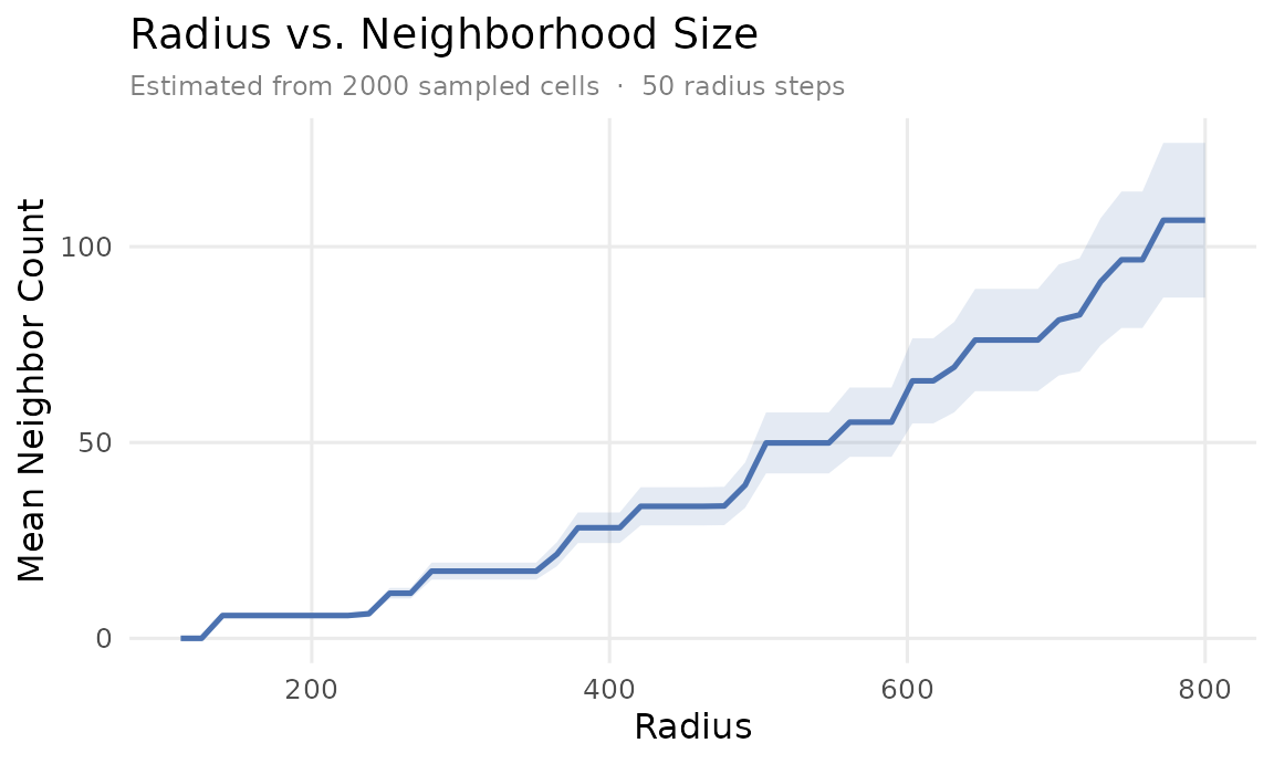
The curve rises in steps because Visium spots sit on a hexagonal
grid. The first step is the ring of 6 touching spots. This tutorial uses
k = 6, which gives those immediate neighbors. Passing
rad instead would use a fixed radius.
This is one tissue section, so sample.col isn’t needed.
Set it when your data has several sections, so that no edges cross
between them.
Build the NICHESObject
Raw counts give scores on an absolute scale. With
"connectomedb2025" you don’t need to download anything
else, and species must match your data.
obj <- create_NICHESObject(
  count.mtx = inputs$count.mtx,
  meta.data = inputs$meta.data,
  LRM.db    = "connectomedb2025",
  species   = "mouse",
  mode      = "spatial",
  k         = 6L,
  method    = "product",
  n.cores   = 2L,
  verbose   = FALSE
)
dim(obj)
#> cells genes edges  LRMs
#>  2696 31053 18500  3097
There’s one row in $edge.data for each non-zero (edge,
LR pair) score:
| edge | LRM | score | score.norm |
|---|---|---|---|
| AAACAAGTATCTCCCA-1|AAACAAGTATCTCCCA-1 | Adam15|Itgav | 4 | 0.002 |
| AAACAAGTATCTCCCA-1|AAACAAGTATCTCCCA-1 | Adam23|Itgav | 2 | 0.001 |
| AAACAAGTATCTCCCA-1|AAACAAGTATCTCCCA-1 | Adamts1|Lrp1 | 4 | 0.002 |
Find the strongest signals
Summing across all edges shows which LR pairs dominate. Abundant genes rise to the top, as they do with any magnitude-based score on raw counts.
| LRM | total.score | edges |
|---|---|---|
| Ppia|Bsg | 22,906,784 | 18,316 |
| App|Aplp1 | 11,794,512 | 18,389 |
| Snca|Aplp1 | 5,434,808 | 17,208 |
| Apoe|Lrp1 | 4,286,950 | 17,273 |
| App|Aplp2 | 4,006,297 | 17,971 |
Aggregate by neighborhood
obj <- aggregate_NICHESObject(obj, verbose = FALSE)
agg <- obj$aggregations$neighborhood.edge.agg
This dataset has no cell-type labels, so we leave out
cell.type.col and skip the composition table.
Map a signal onto the tissue
Penk|Ogfr is a useful example, because Penk is
strongly enriched in the striatum. score.in.sum adds up
everything a spot receives from its neighbors for this LR pair.
one.lrm <- agg[LRM == "Penk|Ogfr", .(cell, score.in.sum)]

plot.dt <- merge(
  obj$cell.meta[, .(cell, x, y)],
  one.lrm,
  by = "cell", all.x = TRUE
)
plot.dt[is.na(score.in.sum), score.in.sum := 0]

ggplot(plot.dt[order(score.in.sum)], aes(y, x, color = score.in.sum)) +
  geom_point(size = 0.9) +
  scale_x_continuous(NULL, labels = NULL) +
  scale_y_reverse(NULL, labels = NULL) +
  scale_color_viridis_c(name = "Received", trans = "sqrt") +
  coord_equal() +
  labs(title = "Penk|Ogfr signal received per spot") +
  theme_minimal(base_size = 11) +
  theme(panel.grid = element_blank())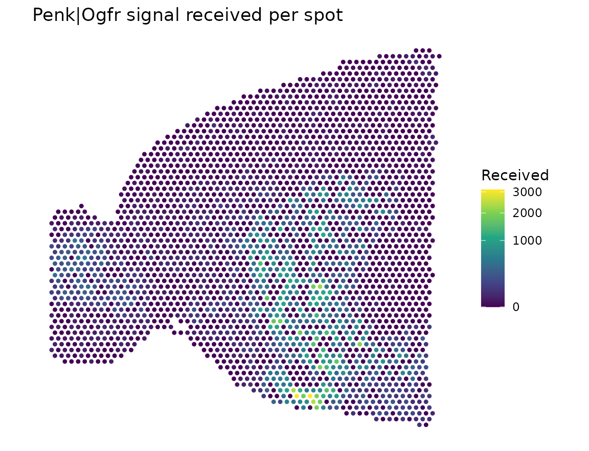
Trace a signal back to its senders
Because every edge is stored, you can see which neighbors sent the
signal to the strongest receiver. share is each sender’s
part of the total.
receiver <- one.lrm[which.max(score.in.sum), cell]

senders <- merge(
  obj$edge.data[LRM == "Penk|Ogfr", .(edge, score)],
  obj$edge.list[ReceivingCell == receiver & SendingCell != receiver],
  by = "edge"
)
senders[, share := score / sum(score)]
senders[order(-score), .(SendingCell, score, share)]| SendingCell | score | share |
|---|---|---|
| AGTACAGAAGCTTATA-1 | 858 | 0.275 |
| ACCGAGTCTCCTTATT-1 | 813 | 0.261 |
| GACCACACTTCCCTTT-1 | 474 | 0.152 |
| TAATACTAGAACAGAC-1 | 414 | 0.133 |
| GGGCAGTCAACGCCAA-1 | 297 | 0.095 |
| GAGATGGCTTTAATCA-1 | 261 | 0.084 |
spots  <- obj$cell.meta[, .(cell, x, y)]
center <- spots[cell == receiver]
nearby <- spots[abs(x - center$x) < 450 & abs(y - center$y) < 450]

arrows <- merge(senders, spots, by.x = "SendingCell", by.y = "cell")
arrows[, `:=`(x.end = x + 0.7 * (center$x - x),
              y.end = y + 0.7 * (center$y - y))]

ggplot() +
  geom_point(data = nearby, aes(y, x), color = "grey85", size = 7) +
  geom_point(data = center, aes(y, x), color = "black", size = 7) +
  geom_segment(
    data = arrows,
    aes(x = y, y = x, xend = y.end, yend = x.end, linewidth = score),
    color = "#1f7a8c",
    arrow = arrow(length = unit(2.5, "mm"), type = "closed")
  ) +
  scale_linewidth(range = c(0.4, 2), name = "Score") +
  scale_x_continuous(NULL, labels = NULL) +
  scale_y_reverse(NULL, labels = NULL) +
  coord_equal() +
  labs(title = "Who sends Penk|Ogfr to the top receiver (black)") +
  theme_minimal(base_size = 11) +
  theme(panel.grid = element_blank())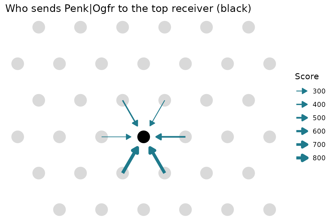
All of these edges share one receiver, so the differences come only from how much Penk each neighbor expresses. Two neighbors supply more than half of the signal.
Export the edges
export_to_TissuePlex() needs the arrow package and
writes one Parquet file.
out.file <- file.path(tempdir(), "edges.parquet")
export_to_TissuePlex(obj, output.path = out.file, celltype.col = NULL)
round(file.size(out.file) / 1e6)
#> [1] 43
The export guide shows what to do with that file.
Data source
The data are from 10x Genomics, “Mouse Brain Serial Section 1
(Sagittal-Anterior)”, Space Ranger 1.0.0, licensed under CC BY 4.0.
NICHESv2 hosts a copy taken from the anterior1 object in
the SeuratData package stxBrain.SeuratData. The copy keeps
the raw counts and spot metadata unchanged, and adds the spot
coordinates. The PROVENANCE.md file that comes with the
download gives the details.